8.2: Precipitation Gravimetry

Last updated
Save as PDF

Page ID: 5702

\( \newcommand{\vecs}[1]{\overset { \scriptstyle \rightharpoonup} {\mathbf{#1}} } \) \( \newcommand{\vecd}[1]{\overset{-\!-\!\rightharpoonup}{\vphantom{a}\smash {#1}}} \)\(\newcommand{\id}{\mathrm{id}}\) \( \newcommand{\Span}{\mathrm{span}}\) \( \newcommand{\kernel}{\mathrm{null}\,}\) \( \newcommand{\range}{\mathrm{range}\,}\) \( \newcommand{\RealPart}{\mathrm{Re}}\) \( \newcommand{\ImaginaryPart}{\mathrm{Im}}\) \( \newcommand{\Argument}{\mathrm{Arg}}\) \( \newcommand{\norm}[1]{\| #1 \|}\) \( \newcommand{\inner}[2]{\langle #1, #2 \rangle}\) \( \newcommand{\Span}{\mathrm{span}}\) \(\newcommand{\id}{\mathrm{id}}\) \( \newcommand{\Span}{\mathrm{span}}\) \( \newcommand{\kernel}{\mathrm{null}\,}\) \( \newcommand{\range}{\mathrm{range}\,}\) \( \newcommand{\RealPart}{\mathrm{Re}}\) \( \newcommand{\ImaginaryPart}{\mathrm{Im}}\) \( \newcommand{\Argument}{\mathrm{Arg}}\) \( \newcommand{\norm}[1]{\| #1 \|}\) \( \newcommand{\inner}[2]{\langle #1, #2 \rangle}\) \( \newcommand{\Span}{\mathrm{span}}\)\(\newcommand{\AA}{\unicode[.8,0]{x212B}}\)

In precipitation gravimetry an insoluble compound forms when we add a precipitating reagent, or precipitant, to a solution containing our analyte. In most methods the precipitate is the product of a simple metathesis reaction between the analyte and the precipitant; however, any reaction generating a precipitate can potentially serve as a gravimetric method.

Most precipitation gravimetric methods were developed in the nineteenth century, or earlier, often for the analysis of ores. Figure 1.1 in Chapter 1, for example, illustrates a precipitation gravimetric method for the analysis of nickel in ores.

8.2.1 Theory and Practice

All precipitation gravimetric analysis share two important attributes. First, the precipitate must be of low solubility, of high purity, and of known composition if its mass is to accurately reflect the analyte’s mass. Second, the precipitate must be easy to separate from the reaction mixture.

Solubility Considerations

To provide accurate results, a precipitate’s solubility must be minimal. The accuracy of a total analysis technique typically is better than ±0.1%, which means that the precipitate must account for at least 99.9% of the analyte. Extending this requirement to 99.99% ensures that the precipitate’s solubility does not limit the accuracy of a gravimetric analysis.

Total Analysis

A total analysis technique is one in which the analytical signal—mass in this case—is proportional to the absolute amount of analyte in the sample. See Chapter 3 for a discussion of the difference between total analysis techniques and concentration techniques.

We can minimize solubility losses by carefully controlling the conditions under which the precipitate forms. This, in turn, requires that we account for every equilibrium reaction affecting the precipitate’s solubility. For example, we can determine Ag⁺ gravimetrically by adding NaCl as a precipitant, forming a precipitate of AgCl.

\[\mathrm{Ag^+}(aq)+\mathrm{Cl^-}(aq)\rightleftharpoons\mathrm{AgCl}(s)\label{8.1}\]

If this is the only reaction we consider, then we predict that the precipitate’s solubility, S_AgCl, is given by the following Equation.

\[S_\textrm{AgCl}=[\mathrm{Ag^+}]=\dfrac{K_\textrm{sp}}{[\mathrm{Cl^-}]}\label{8.2}\]

Equation \ref{8.2} suggests that we can minimize solubility losses by adding a large excess of Cl^–. In fact, as shown in Figure \(\PageIndex{1}\), adding a large excess of Cl^– increases the precipitate’s solubility.

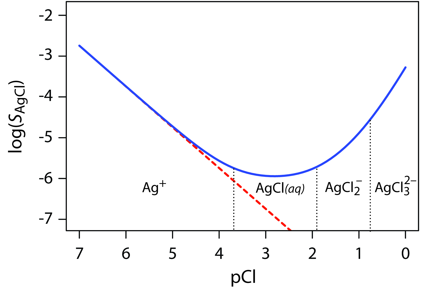
Figure \(\PageIndex{1}\) Solubility of AgCl as a function of pCl. The dashed red line shows our prediction for S_AgCl if we incorrectly assume that only reaction \ref{8.1} and Equation \ref{8.2} affect silver chloride’s solubility. The solid blue curve is calculated using Equation \ref{8.7}, which accounts for reaction \ref{8.1} and reactions 8\(\ref{8.3}–\ref{8.5}. Because the solubility of AgCl spans several orders of magnitude, S_AgCl is displayed on the y-axis in logarithmic form.

To understand why the solubility of AgCl is more complicated than the relationship suggested by Equation \ref{8.2}, we must recognize that Ag⁺ also forms a series of soluble silver-chloro metal–ligand complexes.

\[\mathrm{Ag^+}(aq)+\mathrm{Cl^-}(aq)\rightleftharpoons \mathrm{AgCl}(aq)\hspace{5mm}\log K_1=3.70\label{8.3}\]

\[\mathrm{AgCl}(aq)+\mathrm{Cl^-}(aq)\rightleftharpoons \ce{AgCl_2^-}(aq)\hspace{5mm}\log K_2=1.92\label{8.4}\]

\[\ce{AgCl_2^-}(aq)+\mathrm{Cl^-}(aq)\rightleftharpoons\mathrm{AgCl_3^{2-}}(aq)\hspace{5mm}\log K_3=0.78\label{8.5}\]

The actual solubility of AgCl is the sum of the equilibrium concentrations for all soluble forms of Ag⁺, as shown by the following Equation.

\[S_\textrm{AgCl}=\mathrm{[Ag^+]}+[\mathrm{AgCl}(aq)]+\mathrm{[\ce{AgCl_2^-}]+[AgCl_3^{2-}]}\label{8.6}\]

By substituting into Equation \ref{8.6} the equilibrium constant expressions for reaction \ref{8.1} and reactions \ref{8.3}–\ref{8.5}, we can define the solubility of AgCl as

\[S_\textrm{AgCl}=\dfrac{K_\textrm{sp}}{[\mathrm{Cl^-}]}+K_1K_\textrm{sp}+K_1K_2K_\textrm{sp}[\mathrm{Cl^-}]+K_1K_2K_3K_\textrm{sp}[\mathrm{Cl^-}]^2\label{8.7}\]

Equation \ref{8.7} explains the solubility curve for AgCl shown in Figure \(\PageIndex{1}\). As we add NaCl to a solution of Ag⁺, the solubility of AgCl initially decreases because of reaction \ref{8.1}. Under these conditions, the final three terms in Equation \ref{8.7} are small and Equation \ref{8.1} is sufficient to describe AgCl’s solubility. At higher concentrations of Cl^–, reaction \ref{8.4} and reaction \ref{8.5} increase the solubility of AgCl. Clearly the equilibrium concentration of chloride is important if we want to determine the concentration of silver by precipitating AgCl. In particular, we must avoid a large excess of chloride.

The predominate silver-chloro complexes for different values of pCl are shown by the ladder diagram along the x-axis in Figure \(\PageIndex{1}\) Note that the increase in solubility begins when the higher-order soluble complexes, AgCl₂^– and AgCl₃^2–, become the predominate species.

Another important parameter that may affect a precipitate’s solubility is pH. For example, a hydroxide precipitates such as Fe(OH)₃ is more soluble at lower pH levels where the concentration of OH^– is small. Because fluoride is a weak base, the solubility of calcium fluoride, S_CaF2, also is pH-dependent. We can derive an Equation for S_CaF2 by considering the following equilibrium reactions

\[\mathrm{CaF_2}(s)\rightleftharpoons\mathrm{Ca^{2+}}(aq)+\mathrm{2F^-}(aq){\hspace{5mm}}K_\textrm{sp}=3.9\times10^{-11}\label{8.8}\]

\[\mathrm{HF}(aq)+\mathrm{H_2O}(l)\rightleftharpoons\mathrm{H_3O^+}(aq)+\mathrm{F^-}(aq)\hspace{5mm}K_\textrm a=6.8\times10^{-4}\label{8.9}\]

and the following Equation for the solubility of CaF₂.

\[S_\mathrm{CaF_2}=[\mathrm{Ca^{2+}}]=\dfrac{1}{2}\left\{[\mathrm{F^-}]+[\mathrm{HF}]\right\}\label{8.10}\]

Be sure that Equation \ref{8.10} makes sense to you. Reaction \ref{8.8} tells us that the dissolution of CaF₂ produces one mole of Ca²⁺ for every two moles of F^–, which explains the term of 1/2 in Equation \ref{8.10}. Because F^– is a weak base, we need to account for both of its chemical forms in solution, which explains why we include HF.

Substituting the equilibrium constant expressions for reaction \ref{8.8} and reaction \ref{8.9} into Equation \ref{8.10} defines the solubility of CaF₂ in terms of the equilibrium concentration of H₃O⁺.

\[S_\mathrm{CaF_2}=[\mathrm{Ca^{2+}}]=\left\{\dfrac{K_\textrm{sp}}{4}\left(1+\dfrac{[\mathrm{H_3O^+}]}{K_\textrm a}\right )^2\right\}^{1/3}\label{8.11}\]

Figure \(\PageIndex{2}\) shows how pH affects the solubility of CaF₂. Depending on the solution’s pH, the predominate form of fluoride is either HF or F^–. When the pH is greater than 4.17, the predominate species is F^– and the solubility of CaF₂ is independent of pH because only reaction \ref{8.8} occurs to an appreciable extent. At more acidic pH levels, the solubility of CaF₂ increases because of the contribution of reaction \ref{8.9}.

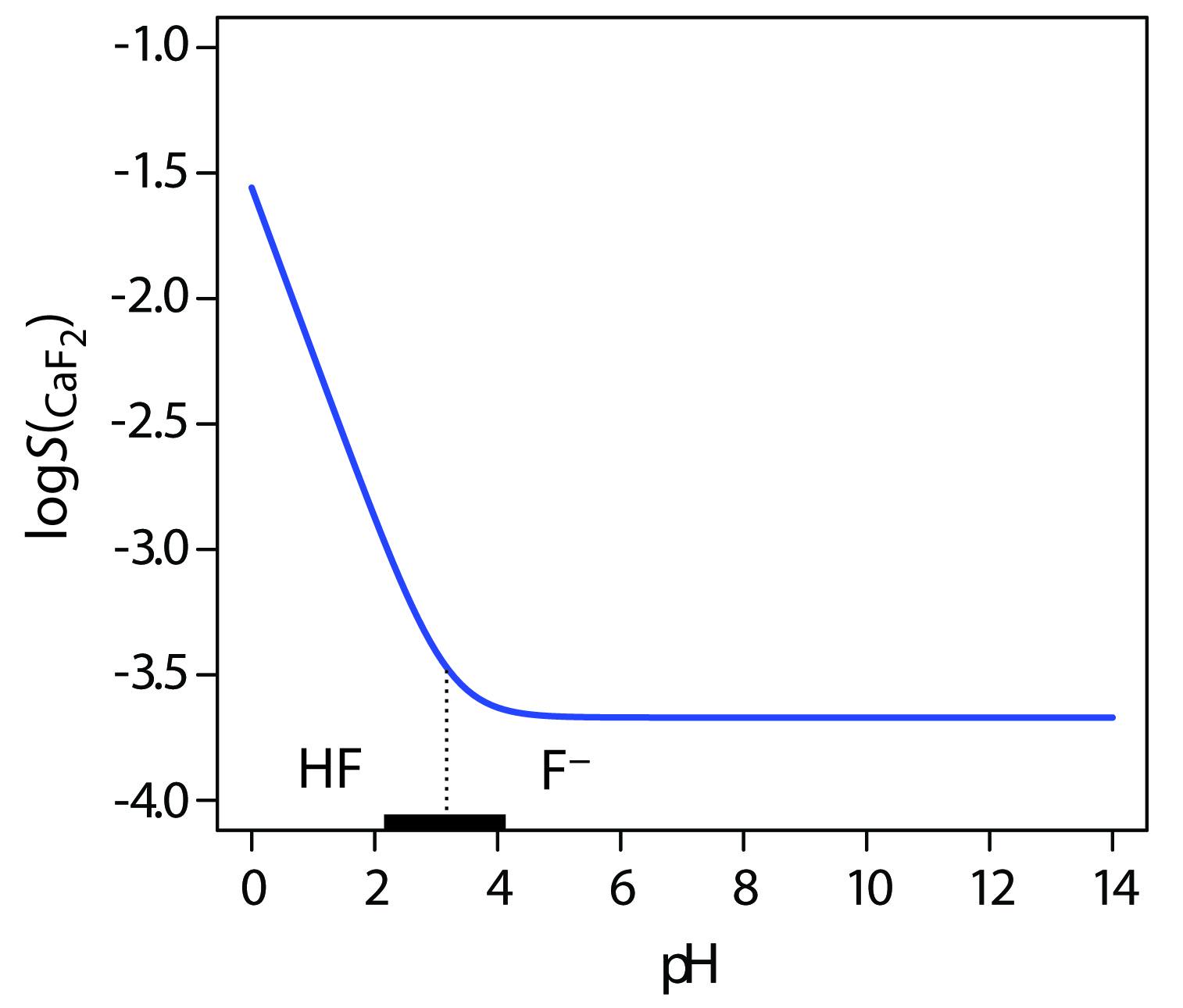
Figure \(\PageIndex{2}\) Solubility of CaF₂ as a function of pH. The solid blue curve is a plot of Equation \ref{8.11}. The predominate form of fluoride in solution is shown by the ladder diagram along the x-axis, with the black rectangle showing the region where both HF and F^– are important species. Note that the solubility of CaF₂ is independent of pH for pH levels greater than 4.17, and that its solubility increases dramatically at lower pH levels where HF is the predominate species. Because the solubility of CaF₂ spans several orders of magnitude, its solubility is shown in logarithmic form.

When solubility is a concern, it may be possible to decrease solubility by using a non-aqueous solvent. A precipitate’s solubility is generally greater in an aqueous solution because of water’s ability to stabilize ions through solvation. The poorer solvating ability of non-aqueous solvents, even those which are polar, leads to a smaller solubility product. For example, the K_sp of PbSO₄ is 2 × 10^–8 in H₂O and 2.6 × 10^–12 in a 50:50 mixture of H₂O and ethanol.

Exercise 8.1

You can use a ladder diagram to predict the conditions for minimizing a precipitate’s solubility. Draw a ladder diagram for oxalic acid, H₂C₂O₄, and use it to establish a suitable range of pH values for minimizing the solubility of CaC₂O₄. Relevant equilibrium constants may be found in the appendices.

Click here to review your answer to this exercise.

Avoiding Impurities

In addition to having a low solubility, the precipitate must be free from impurities. Because precipitation usually occurs in a solution that is rich in dissolved solids, the initial precipitate is often impure. We must remove these impurities before determining the precipitate’s mass.

The greatest source of impurities is the result of chemical and physical interactions occurring at the precipitate’s surface. A precipitate is generally crystalline—even if only on a microscopic scale—with a well-defined lattice of cations and anions. Those cations and anions at the precipitate’s surface carry, respectively, a positive or a negative charge because they have incomplete coordination spheres. In a precipitate of AgCl, for example, each silver ion in the precipitate’s interior is bound to six chloride ions. A silver ion at the surface, however, is bound to no more than five chloride ions and carries a partial positive charge (Figure \(\PageIndex{3}\)). The presence of these partial charges makes the precipitate’s surface an active site for the chemical and physical interactions that produce impurities.

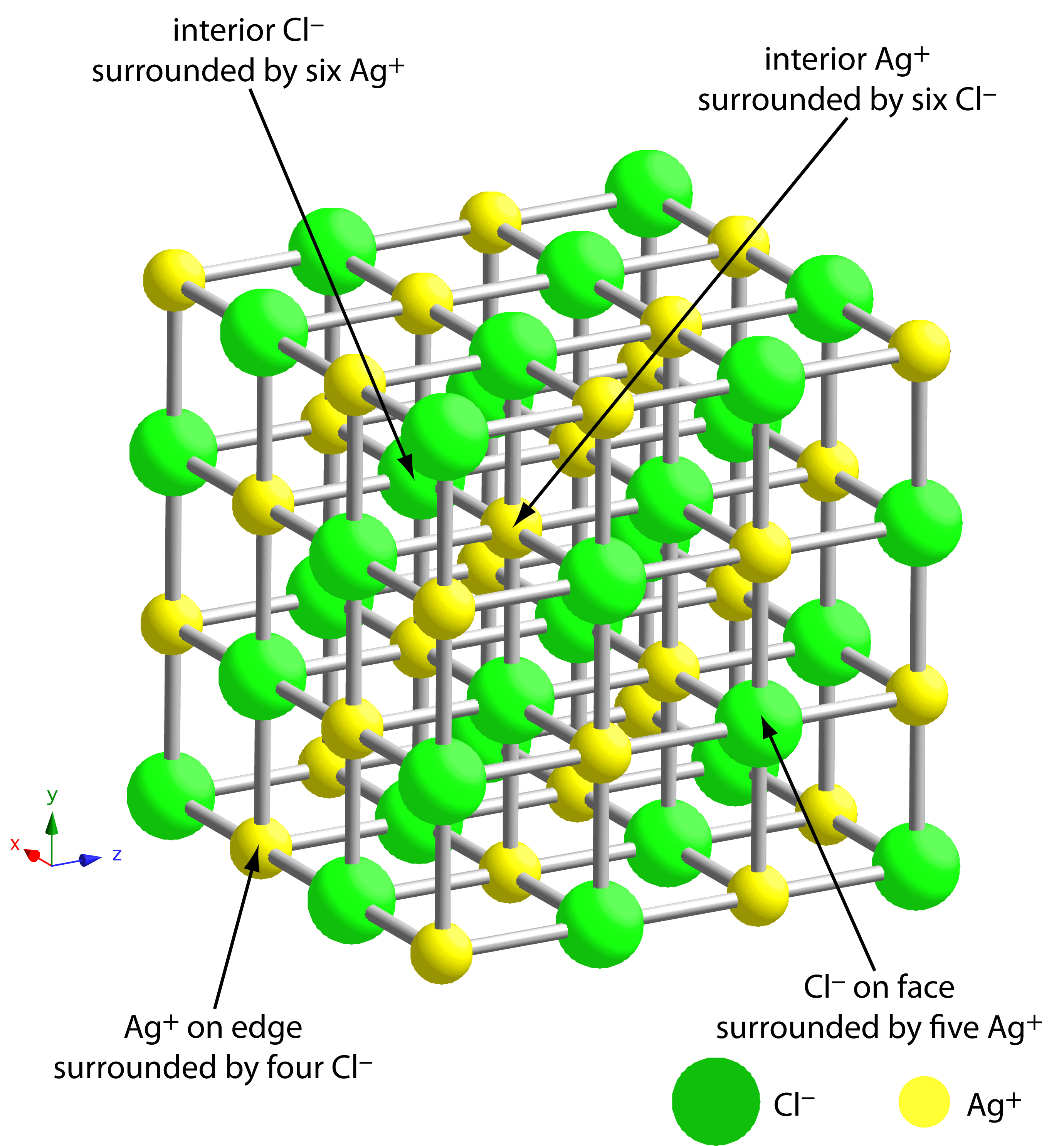
Figure \(\PageIndex{3}\): Ball-and-stick diagram showing the lattice structure of AgCl. Each silver ion in the lattice’s interior binds with six chloride ions, and each chloride ion in the interior binds with six silver ions. Those ions on the lattice’s surface or edges bind to fewer than six ions and carry a partial charge. A silver ion on the surface, for example, carries a partial positive charge. These charges make the surface of a precipitate an active site for chemical and physical interactions.

One common impurity is an inclusion. A potential interfering ion whose size and charge is similar to a lattice ion, may substitute into the lattice structure, provided that the interferent precipitates with the same crystal structure (Figure \(\PageIndex{4}\)a). The probability of forming an inclusion is greatest when the concentration of the interfering ion is substantially greater than the lattice ion’s concentration. An inclusion does not decrease the amount of analyte that precipitates, provided that the precipitant is present in sufficient excess. Thus, the precipitate’s mass is always larger than expected.

Figure \(\PageIndex{4}\) Three examples of impurities that may form during precipitation. The cubic frame represents the precipitate and the blue marks are impurities: (a) inclusions, (b) occlusions, and (c) surface adsorbates. Inclusions are randomly distributed throughout the precipitate. Occlusions are localized within the interior of the precipitate and surface adsorbates are localized on the precipitate’s exterior. For ease of viewing, in (c) adsorption is shown on only one surface.

An inclusion is difficult to remove since it is chemically part of the precipitate’s lattice. The only way to remove an inclusion is through reprecipitation. After isolating the precipitate from its supernatant solution, we dissolve it by heating in a small portion of a suitable solvent. We then allow the solution to cool, reforming the precipitate. Because the interferent’s concentration is less than that in the original solution, the amount of included material is smaller. We can repeat the process of reprecipitation until the inclusion’s mass is insignificant. The loss of analyte during reprecipitation, however, can be a significant source of error.

Suppose that 10% of an interferent forms an inclusion during each precipitation. When we initially form the precipitate, 10% of the original interferent is present as an inclusion. After the first reprecipitation, 10% of the included interferent remains, which is 1% of the original interferent. A second reprecipitation decreases the interferent to 0.1% of the original amount.

Occlusions form when interfering ions become trapped within the growing precipitate. Unlike inclusions, which are randomly dispersed within the precipitate, an occlusion is localized, either along flaws within the precipitate’s lattice structure or within aggregates of individual precipitate particles (Figure \(\PageIndex{4}\)b). An occlusion usually increases a precipitate’s mass; however, the mass is smaller if the occlusion includes the analyte in a lower molecular weight form than that of the precipitate.

We can minimize occlusions by maintaining the precipitate in equilibrium with its supernatant solution for an extended time. This process is called a digestion. During digestion, the dynamic nature of the solubility–precipitation equilibrium, in which the precipitate dissolves and reforms, ensures that the occlusion is reexposed to the supernatant solution. Because the rates of dissolution and reprecipitation are slow, there is less opportunity for forming new occlusions.

After precipitation is complete the surface continues to attract ions from solution (Figure \(\PageIndex{4}\)c). These surface adsorbates comprise a third type of impurity. We can minimize surface adsorption by decreasing the precipitate’s available surface area. One benefit of digesting a precipitate is that it increases the average particle size. Because the probability of a particle completely dissolving is inversely proportional to its size, during digestion larger particles increase in size at the expense of smaller particles. One consequence of forming a smaller number of larger particles is an overall decrease in the precipitate’s surface area. We also can remove surface adsorbates by washing the precipitate, although the potential loss of analyte can not be ignored.

Inclusions, occlusions, and surface adsorbates are examples of coprecipitates—otherwise soluble species that form within the precipitate containing the analyte. Another type of impurity is an interferent that forms an independent precipitate under the conditions of the analysis. For example, the precipitation of nickel dimethylglyoxime requires a slightly basic pH. Under these conditions, any Fe³⁺ in the sample precipitates as Fe(OH)₃. In addition, because most precipitants are rarely selective toward a single analyte, there is always a risk that the precipitant will react with both the analyte and an interferent.

In addition to forming a precipitate with Ni²⁺, dimethylglyoxime also forms precipitates with Pd²⁺ and Pt²⁺. These cations are potential interferents in an analysis for nickel.

We can minimize the formation of additional precipitates by carefully controlling solution conditions. If an interferent forms a precipitate that is less soluble than the analyte’s precipitate, we can precipitate the interferent and remove it by filtration, leaving the analyte behind in solution. Alternatively, we can mask the analyte or the interferent to prevent its precipitation.

Both of the above-mentioned approaches are illustrated in Fresenius’ analytical method for determining Ni in ores containing Pb²⁺, Cu²⁺, and Fe³⁺ (Figure 1.1 in Chapter 1). Dissolving the ore in the presence of H₂SO₄ selectively precipitates Pb²⁺ as PbSO₄. Treating the supernatant with H₂S precipitates the Cu²⁺ as CuS. After removing the CuS by filtration, adding ammonia precipitates Fe³⁺ as Fe(OH)₃. Nickel, which forms a soluble amine complex, remains in solution.

Controlling Particle Size

Size matters when it comes to forming a precipitate. Larger particles are easier to filter, and, as noted earlier, a smaller surface area means there is less opportunity for surface adsorbates to form. By carefully controlling the reaction conditions we can significantly increase a precipitate’s average particle size.

Precipitation consists of two distinct events: nucleation, the initial formation of smaller stable particles of precipitate, and particle growth. Larger particles form when the rate of particle growth exceeds the rate of nucleation. Understanding the conditions favoring particle growth is important when designing a gravimetric method of analysis.

We define a solute’s relative supersaturation, RSS, as

\[RSS=\dfrac{Q-S}{S}\label{8.12}\]

where Q is the solute’s actual concentration and S is the solute’s concentration at equilibrium.⁴ The numerator of Equation \ref{8.12}, Q – S, is a measure of the solute’s supersaturation. A solution with a large, positive value of RSS has a high rate of nucleation, producing a precipitate with many small particles. When the RSS is small, precipitation is more likely to occur by particle growth than by nucleation.

A supersaturated solution is one that contains more dissolved solute than that predicted by equilibrium chemistry. The solution is inherently unstable and precipitates solute to reach its equilibrium position. How quickly this process occurs depends, in part, on the value of RSS.

Examining Equation \ref{8.12} shows that we can minimize RSS by decreasing the solute’s concentration, Q, or by increasing the precipitate’s solubility, S. A precipitate’s solubility usually increases at higher temperatures, and adjusting pH may affect a precipitate’s solubility if it contains an acidic or a basic ion. Temperature and pH, therefore, are useful ways to increase the value of S. Conducting the precipitation in a dilute solution of analyte, or adding the precipitant slowly and with vigorous stirring are ways to decrease the value of Q.

There are practical limitations to minimizing RSS. Some precipitates, such as Fe(OH)₃ and PbS, are so insoluble that S is very small and a large RSS is unavoidable. Such solutes inevitably form small particles. In addition, conditions favoring a small RSS may lead to a relatively stable supersaturated solution that requires a long time to fully precipitate. For example, almost a month is required to form a visible precipitate of BaSO₄ under conditions in which the initial RSS is 5.⁵

A visible precipitate takes longer to form when RSS is small both because there is a slow rate of nucleation and because there is a steady decrease in RSS as the precipitate forms. One solution to the latter problem is to generate the precipitant in situ as the product of a slow chemical reaction. This maintains the RSS at an effectively constant level. Because the precipitate forms under conditions of low RSS, initial nucleation produces a small number of particles. As additional precipitant forms, particle growth supersedes nucleation, resulting in larger precipitate particles. This process is called homogeneous precipitation.⁶

Two general methods are used for homogeneous precipitation. If the precipitate’s solubility is pH-dependent, then we can mix the analyte and the precipitant under conditions where precipitation does not occur, and then increase or decrease the pH by chemically generating OH^– or H₃O⁺. For example, the hydrolysis of urea is a source of OH^–.

\[\mathrm{CO(NH_2)_2}(aq)+\mathrm{H_2O}(l)\rightleftharpoons\mathrm{2NH_3}(aq)+\mathrm{CO_2}(g)\]

\[\mathrm{NH_3}(aq)+\mathrm{H_2O}(l)\rightleftharpoons\mathrm{OH^-}(aq)+\mathrm{NH_4^+}(aq)\]

Because the hydrolysis of urea is temperature-dependent—it is negligible at room temperature—we can use temperature to control the rate of hydrolysis and the rate of precipitate formation. Precipitates of CaC₂O₄, for example, have been produced by this method. After dissolving the sample containing Ca²⁺, the solution is made acidic with HCl before adding a solution of 5% w/v (NH₄)₂C₂O₄. Because the solution is acidic, a precipitate of CaC₂O₄ does not form. The solution is heated to approximately 50^oC and urea is added. After several minutes, a precipitate of CaC₂O₄ begins to form, with precipitation reaching completion in about 30 min.

In the second method of homogeneous precipitation, the precipitant is generated by a chemical reaction. For example, Pb²⁺ is precipitated homogeneously as PbCrO₄ by using bromate, BrO₃^–, to oxidize Cr³⁺ to CrO₄^2–.

\[\ce{6BrO_3^-}(aq)+\mathrm{10Cr^{3+}}(aq)+\mathrm{22H_2O}(l)\rightleftharpoons\mathrm{3Br_2}(aq)+\mathrm{10CrO_4^{2-}}(aq)+\mathrm{44H^+}(aq)\]

Figure \(\PageIndex{5}\) shows the result of preparing PbCrO₄ by the direct addition of KCrO₄ (Beaker A) and by homogenous precipitation (Beaker B). Both beakers contain the same amount of PbCrO₄. Because the direct addition of KCrO₄ leads to rapid precipitation and the formation of smaller particles, the precipitate remains less settled than the precipitate prepared homogeneously. Note, as well, the difference in the color of the two precipitates.

Figure \(\PageIndex{5}\) Two precipitates of PbCrO₄. In Beaker A, combining 0.1 M Pb(NO₃)₂ and 0.1 M K₂CrO₄ forms the precipitate under conditions of high RSS. The precipitate forms rapidly and consists of very small particles. In Beaker B, heating a solution of 0.1 M Pb(NO₃)₂, 0.1 M Cr(NO₃)₃, and 0.1 M KBrO₃ slowly oxidizes Cr³⁺ to CrO₄^2–, precipitating PbCrO₄ under conditions of low RSS. The precipitate forms slowly and consists of much larger particles.

The effect of particle size on color is well-known to geologists, who use a streak test to help identify minerals. The color of a bulk mineral and its color when powdered are often different. Rubbing a mineral across an unglazed porcelain plate leaves behind a small streak of the powdered mineral. Bulk samples of hematite, Fe₂O₃, are black in color, but its streak is a familiar rust-red. Crocite, the mineral PbCrO₄, is red-orange in color; its streak is orange-yellow.

A homogeneous precipitation produces large particles of precipitate that are relatively free from impurities. These advantages, however, are offset by requiring more time to produce the precipitate and a tendency for the precipitate to deposit as a thin film on the container’s walls. The latter problem is particularly severe for hydroxide precipitates generated using urea.

An additional method for increasing particle size deserves mention. When a precipitate’s particles are electrically neutral they tend to coagulate into larger particles that are easier to filter. Surface adsorption of excess lattice ions, however, provides the precipitate’s particles with a net positive or a net negative surface charge. Electrostatic repulsion between the particles prevents them from coagulating into larger particles.

Let’s use the precipitation of AgCl from a solution of AgNO₃ using NaCl as a precipitant to illustrate this effect. Early in the precipitation, when NaCl is the limiting reagent, excess Ag⁺ ions chemically adsorb to the AgCl particles, forming a positively charged primary adsorption layer (Figure \(\PageIndex{6}\)a). The solution in contact with this layer contains more inert anions, NO₃^– in this case, than inert cations, Na⁺, giving a secondary adsorption layer with a negative charge that balances the primary adsorption layer’s positive charge. The solution outside the secondary adsorption layer remains electrically neutral. Coagulation cannot occur if the secondary adsorption layer is too thick because the individual particles of AgCl are unable to approach each other closely enough.

Figure \(\PageIndex{6}\) Two methods for coagulating a precipitate of AgCl. (a) Coagulation does not happen due to the electrostatic repulsion between the two positively charged particles. (b) Decreasing the charge within the primary adsorption layer, by adding additional NaCl, decreases the electrostatic repulsion, allowing the particles to coagulate. (c) Adding additional inert ions decreases the thickness of the secondary adsorption layer. Because the particles can approach each other more closely, they are able to coagulate.

We can induce coagulation in three ways: by decreasing the number of chemically adsorbed Ag⁺ ions, by increasing the concentration of inert ions, or by heating the solution. As we add additional NaCl, precipitating more of the excess Ag⁺, the number of chemically adsorbed silver ions decreases and coagulation occurs (Figure \(\PageIndex{6}\)b). Adding too much NaCl, however, creates a primary adsorption layer of excess Cl^– with a loss of coagulation.

The coagulation and decoagulation of AgCl as we add NaCl to a solution of AgNO₃ can serve as an endpoint for a titration. See Chapter 9 for additional details.

A second way to induce coagulation is to add an inert electrolyte, which increases the concentration of ions in the secondary adsorption layer. With more ions available, the thickness of the secondary absorption layer decreases. Particles of precipitate may now approach each other more closely, allowing the precipitate to coagulate. The amount of electrolyte needed to cause spontaneous coagulation is called the critical coagulation concentration.

Heating the solution and precipitate provides a third way to induce coagulation. As the temperature increases, the number of ions in the primary adsorption layer decreases, lowering the precipitate’s surface charge. In addition, heating increases the particles’ kinetic energy, allowing them to overcome the electrostatic repulsion that prevents coagulation at lower temperatures.

Filtering the Precipitate

After precipitating and digesting the precipitate, we separate it from solution by filtering. The most common filtration method uses filter paper, which is classified according to its speed, its size, and its ash content on ignition. Speed, or how quickly the supernatant passes through the filter paper, is a function of the paper’s pore size. A larger pore allows the supernatant to pass more quickly through the filter paper, but does not retain small particles of precipitate. Filter paper is rated as fast (retains particles larger than 20–25 μm), medium–fast (retains particles larger than 16 μm), medium (retains particles larger than 8 μm), and slow (retains particles larger than 2–3 μm). The proper choice of filtering speed is important. If the filtering speed is too fast, we may fail to retain some of the precipitate, causing a negative determinate error. On the other hand, the precipitate may clog the pores if we use a filter paper that is too slow.

A filter paper’s size is just its diameter. Filter paper comes in many sizes, including 4.25 cm, 7.0 cm, 11.0 cm, 12.5 cm, 15.0 cm, and 27.0 cm. Choose a size that fits comfortably into your funnel. For a typical 65-mm long-stem funnel, 11.0 cm and 12.5 cm filter paper are good choices.

Because filter paper is hygroscopic, it is not easy to dry it to a constant weight. When accuracy is important, the filter paper is removed before determining the precipitate’s mass. After transferring the precipitate and filter paper to a covered crucible, we heat the crucible to a temperature that coverts the paper to CO₂(g) and H₂O(g), a process called ignition.

Igniting a poor quality filter paper leaves behind a residue of inorganic ash. For quantitative work, use a low-ash filter paper. This grade of filter paper is pretreated with a mixture of HCl and HF to remove inorganic materials. Quantitative filter paper typically has an ash content of less than 0.010% w/w.

Gravity filtering is accomplished by folding the filter paper into a cone and placing it in a long-stem funnel (Figure \(\PageIndex{7}\)). A seal between the filter cone and the funnel is formed by dampening the paper with water or supernatant, and pressing the paper to the wall of the funnel. When properly prepared, the funnel’s stem fills with the supernatant, increasing the rate of filtration.

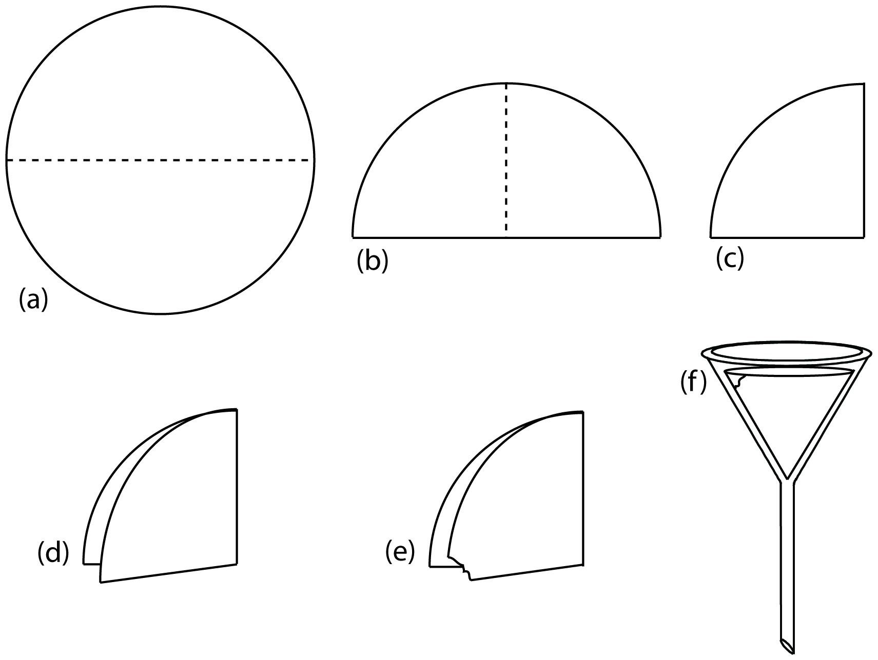
Figure \(\PageIndex{7}\): Preparing a filter paper cone. The filter paper circle in (a) is folded in half (b), and folded in half again (c). The folded filter paper is parted (d) and a small corner is torn off (e). The filter paper is opened up into a cone and placed in the funnel (f ).

The precipitate is transferred to the filter in several steps. The first step is to decant the majority of the supernatant through the filter paper without transferring the precipitate (Figure \(\PageIndex{8}\)). This prevents the filter paper from clogging at the beginning of the filtration process. The precipitate is rinsed while it remains in its beaker, with the rinsings decanted through the filter paper. Finally, the precipitate is transferred onto the filter paper using a stream of rinse solution. Any precipitate clinging to the walls of the beaker is transferred using a rubber policeman (a flexible rubber spatula attached to the end of a glass stirring rod).

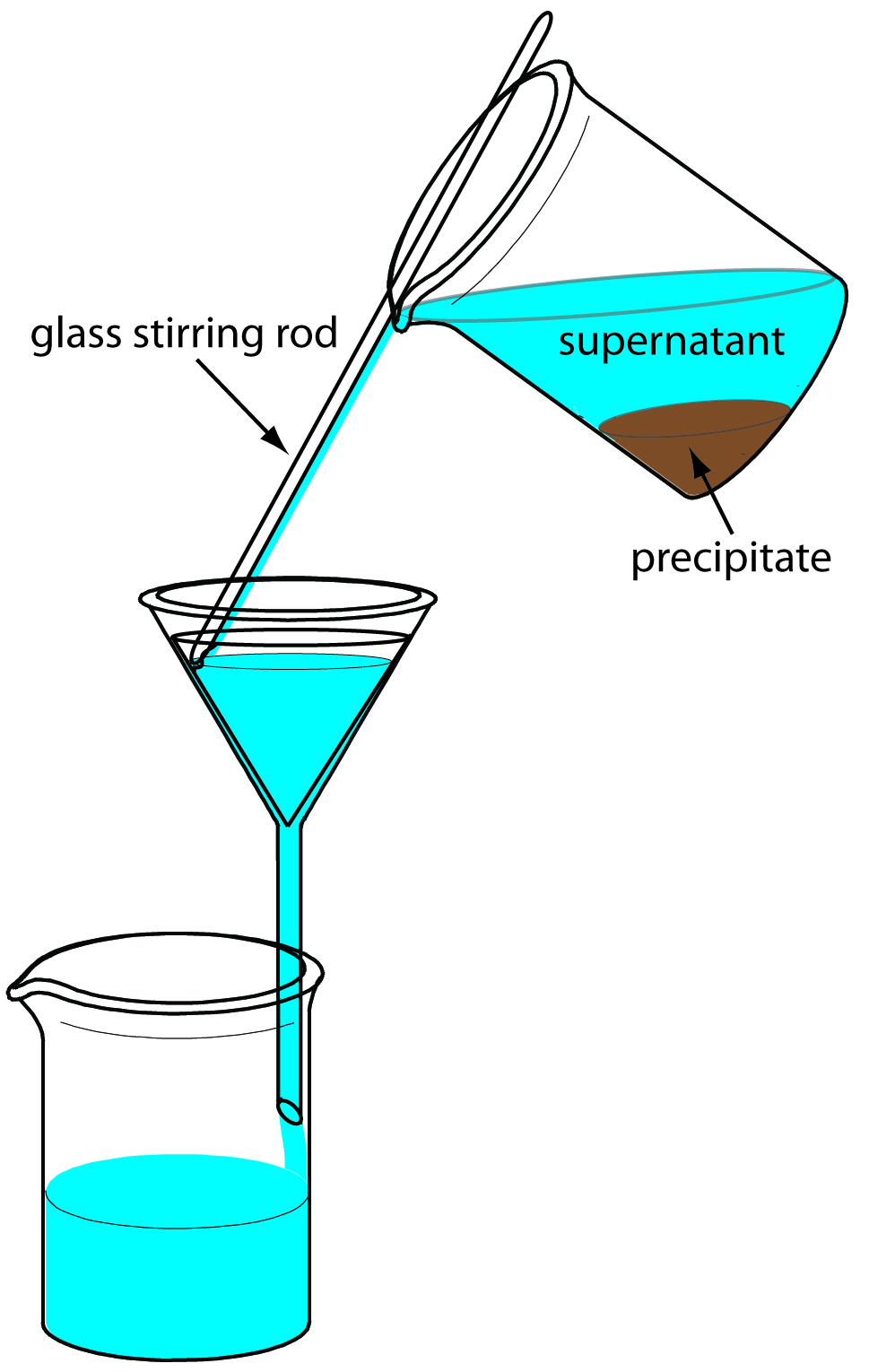
Figure \(\PageIndex{8}\): Proper procedure for transferring the supernatant to the filter paper cone.

An alternative method for filtering a precipitate is a filtering crucible. The most common is a fritted-glass crucible containing a porous glass disk filter. Fritted-glass crucibles are classified by their porosity: coarse (retaining particles larger than 40–60 μm), medium (retaining particles greater than 10–15 μm), and fine (retaining particles greater than 4–5.5 μm). Another type of filtering crucible is the Gooch crucible, which is a porcelain crucible with a perforated bottom. A glass fiber mat is placed in the crucible to retain the precipitate. For both types of crucibles, the precipitate is transferred in the same manner described earlier for filter paper. Instead of using gravity, the supernatant is drawn through the crucible with the assistance of suction from a vacuum aspirator or pump (Figure \(\PageIndex{9}\)).

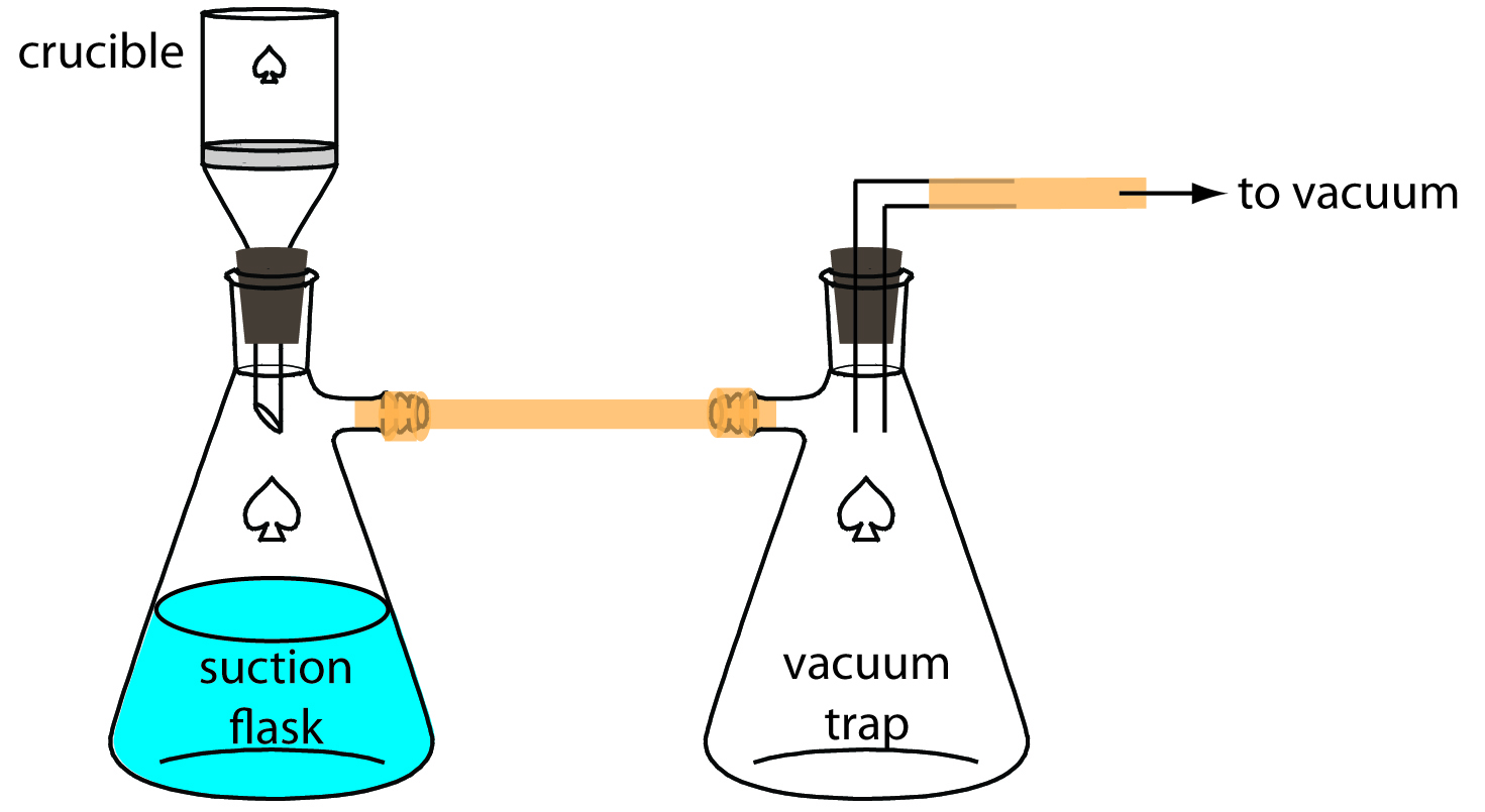
Figure \(\PageIndex{9}\): Procedure for filtering a precipitate through a filtering crucible. The trap prevents water from an aspirator from back-washing into the suction flask.

Rinsing the Precipitate

Because the supernatant is rich with dissolved inert ions, we must remove any residual traces of supernatant to avoid a positive determinate error without incurring solubility losses. In many cases this simply involves the use of cold solvents or rinse solutions containing organic solvents such as ethanol. The pH of the rinse solution is critical if the precipitate contains an acidic or basic ion. When coagulation plays an important role in determining particle size, adding a volatile inert electrolyte to the rinse solution prevents the precipitate from reverting into smaller particles that might pass through the filter. This process of reverting to smaller particles is called peptization. The volatile electrolyte is removed when drying the precipitate.

In general, we can minimize the loss of analyte by using several small portions of rinse solution instead of a single large volume. Testing the used rinse solution for the presence of impurities is another way to guard against over rinsing the precipitate. For example, if Cl^– is a residual ion in the supernatant, we can test for its presence using AgNO₃. After collecting a small portion of the rinse solution, we add a few drops of AgNO₃ and look for the presence or absence of a precipitate of AgCl. If a precipitate forms, then we know that Cl^– is present and continue to rinse the precipitate. Additional rinsing is not needed if the AgNO₃ does not produce a precipitate.

Drying the Precipitate

After separating the precipitate from its supernatant solution, the precipitate is dried to remove residual traces of rinse solution and any volatile impurities. The temperature and method of drying depend on the method of filtration and the precipitate’s desired chemical form. Placing the precipitate in a laboratory oven and heating to a temperature of 110^oC is sufficient when removing water and other easily volatilized impurities. Higher temperatures require a muffle furnace, a Bunsen burner, or a Meker burner, and are necessary if we need to thermally decompose the precipitate before weighing.

Because filter paper absorbs moisture, we must remove it before weighing the precipitate. This is accomplished by folding the filter paper over the precipitate and transferring both the filter paper and the precipitate to a porcelain or platinum crucible. Gentle heating first dries and then chars the filter paper. Once the paper begins to char, we slowly increase the temperature until all traces of the filter paper are gone and any remaining carbon is oxidized to CO₂.

Fritted-glass crucibles can not withstand high temperatures and must be dried in an oven at temperatures below 200^oC. The glass fiber mats used in Gooch crucibles can be heated to a maximum temperature of approximately 500^oC.

Composition of the Final Precipitate

For a quantitative application, the final precipitate must have a well-defined composition. Precipitates containing volatile ions or substantial amounts of hydrated water, are usually dried at a temperature that completely removes these volatile species. For example, one standard gravimetric method for the determination of magnesium involves its precipitation as MgNH₄PO₄•6H₂O. Unfortunately, this precipitate is difficult to dry at lower temperatures without losing an inconsistent amount of hydrated water and ammonia. Instead, the precipitate is dried at temperatures above 1000^oC where it decomposes to magnesium pyrophosphate, Mg₂P₂O₇.

An additional problem is encountered if the isolated solid is nonstoichiometric. For example, precipitating Mn²⁺ as Mn(OH)₂ and heating frequently produces a nonstoichiometric manganese oxide, MnO_x, where x varies between one and two. In this case the nonstoichiometric product is the result of forming of a mixture of oxides with different oxidation state of manganese. Other nonstoichiometric compounds form as a result of lattice defects in the crystal structure.⁷

The best way to appreciate the theoretical and practical details discussed in this section is to carefully examine a typical precipitation gravimetric method. Although each method is unique, the determination of Mg²⁺ in water and wastewater by precipitating MgNH₄PO₄ • 6H₂O and isolating Mg₂P₂O₇ provides an instructive example of a typical procedure. The description here is based on Method 3500-Mg D in Standard Methods for the Examination of Water and Wastewater, 19th Ed., American Public Health Association: Washington, D. C., 1995. With the publication of the 20th Edition in 1998, this method is no longer listed as an approved method.

Representative Method \(\PageIndex{1}\): Determination of Mg²⁺ in Water and Wastewater

Description of Method

Magnesium is precipitated as MgNH₄PO₄ • 6H₂O using (NH₄)₂HPO₄ as the precipitant. The precipitate’s solubility in neutral solutions is relatively high (0.0065 g/100 mL in pure water at 10^oC), but it is much less soluble in the presence of dilute ammonia (0.0003 g/100 mL in 0.6 M NH₃). Because the precipitant is not selective, a preliminary separation of Mg²⁺ from potential interferents is necessary. Calcium, which is the most significant interferent, is removed by precipitating it as CaC₂O₄. The presence of excess ammonium salts from the precipitant, or the addition of too much ammonia leads to the formation of Mg(NH₄)₄(PO₄)₂, which forms Mg(PO₃)₂ after drying. The precipitate is isolated by filtering, using a rinse solution of dilute ammonia. After filtering, the precipitate is converted to Mg₂P₂O₇ and weighed.

Procedure

Transfer a sample containing no more than 60 mg of Mg²⁺ into a 600-mL beaker. Add 2–3 drops of methyl red indicator, and, if necessary, adjust the volume to 150 mL. Acidify the solution with 6 M HCl and add 10 mL of 30% w/v (NH₄)₂HPO₄. After cooling and with constant stirring, add concentrated NH₃ dropwise until the methyl red indicator turns yellow (pH > 6.3). After stirring for 5 min, add 5 mL of concentrated NH₃ and continue stirring for an additional 10 min. Allow the resulting solution and precipitate to stand overnight. Isolate the precipitate by filtering through filter paper, rinsing with 5% v/v NH₃. Dissolve the precipitate in 50 mL of 10% v/v HCl, and precipitate a second time following the same procedure. After filtering, carefully remove the filter paper by charring. Heat the precipitate at 500^oC until the residue is white, and then bring the precipitate to constant weight at 1100^oC.

Questions

1. Why does the procedure call for a sample containing no more than 60 mg of Mg²⁺?

A 60-mg portion of Mg²⁺ generates approximately 600 mg of MgNH₄PO₄ • 6H₂O. This is a substantial amount of precipitate. A larger quantity of precipitate may be difficult to filter and difficult to adequately rinse free of impurities.

2. Why is the solution acidified with HCl before adding the precipitant?

The HCl ensures that MgNH₄PO₄ • 6H₂O does not immediately precipitate when adding the precipitant. Because PO₄^3– is a weak base, the precipitate is soluble in a strongly acidic solution. If the precipitant is added under neutral or basic conditions (high RSS) the resulting precipitate consists of smaller, less pure particles. Increasing the pH by adding base allows the precipitate to form under more favorable (low RSS) conditions.

3. Why is the acid–base indicator methyl red added to the solution?

The indicator’s color change, which occurs at a pH of approximately 6.3, indicates when there is sufficient NH₃ to neutralize the HCl added at the beginning of the procedure. The amount of NH₃ is crucial to this procedure. If we add insufficient NH₃, then the solution is too acidic, which increases the precipitate’s solubility and leads to a negative determinate error. If we add too much NH₃, the precipitate may contain traces of Mg(NH₄)₄(PO₄)₂, which, on drying, forms Mg(PO₃)₂ instead of Mg₂P₂O₇. This increases the mass of the ignited precipitate, giving a positive determinate error. After adding enough NH₃ to neutralize the HCl, we add the additional 5 mL of NH₃ to quantitatively precipitate MgNH₄PO₄ • 6H₂O.

4. Explain why forming Mg(PO₃)₂ instead of Mg₂P₂O₇ increases the precipitate’s mass.

Each mole of Mg₂P₂O₇ contains two moles of phosphorous and each mole of Mg(PO₃)₂ contains only one mole of phosphorous A conservation of mass, therefore, requires that two moles of Mg(PO₃)₂ form in place of each mole of Mg₂P₂O₇. One mole of Mg₂P₂O₇ weighs 222.6 g. Two moles of Mg(PO₃)₂ weigh 364.5 g. Any replacement of Mg₂P₂O₇ with Mg(PO₃)₂ must increase the precipitate’s mass.

5. What additional steps, beyond those discussed in questions 2 and 3, help improve the precipitate’s purity?

Two additional steps in the procedure help in forming a precipitate that is free of impurities: digestion and reprecipitation.

6. Why is the precipitate rinsed with a solution of 5% v/v NH₃?

This is done for the same reason that precipitation is carried out in an ammonical solution; using dilute ammonia minimizes solubility losses when rinsing the precipitate.

8.2.2 Quantitative Applications

Although no longer a commonly used technique, precipitation gravimetry still provides a reliable means for assessing the accuracy of other methods of analysis, or for verifying the composition of standard reference materials. In this section we review the general application of precipitation gravimetry to the analysis of inorganic and organic compounds.

Inorganic Analysis

Table \(\PageIndex{1}\) provides a summary of some precipitation gravimetric methods for inorganic cations and anions. Several methods for the homogeneous generation of precipitants are shown in Table \(\PageIndex{2}\). The majority of inorganic precipitants show poor selectivity for the analyte. Many organic precipitants, however, are selective for one or two inorganic ions. Table \(\PageIndex{3}\) lists several common organic precipitants.

Precipitation gravimetry continues to be listed as a standard method for the determination of SO₄^2– in water and wastewater analysis.⁸ Precipitation is carried out using BaCl₂ in an acidic solution (adjusted with HCl to a pH of 4.5–5.0) to prevent the possible precipitation of BaCO₃ or Ba₃(PO₄)₂, and near the solution’s boiling point. The precipitate is digested at 80–90^oC for at least two hours. Ashless filter paper pulp is added to the precipitate to aid in filtration. After filtering, the precipitate is ignited to constant weight at 800^oC. Alternatively, the precipitate is filtered through a fine porosity fritted glass crucible (without adding filter paper pulp), and dried to constant weight at 105^oC. This procedure is subject to a variety of errors, including occlusions of Ba(NO₃)₂, BaCl₂, and alkali sulfates.

**Table \(\PageIndex{1}\):** Selected Precipitation Gravimetric Methods for Inorganic Cations and Anions (Arranged by Precipitant)
Analyte	Precipitant	Precipitate Formed	Precipitate Weighed
Ba²⁺	(NH₄)₂CrO₄	BaCrO₄	BaCrO₄
Pb²⁺	K₂CrO₄	PbCrO₄	PbCrO₄
Ag⁺	HCl	AgCl	AgCl
Hg₂²⁺	HCl	Hg₂Cl₂	Hg₂Cl₂
Al³⁺	NH₃	Al(OH)₃	Al₂O₃
Be²⁺	NH₃	Be(OH)₂	BeO
Fe³⁺	NH₃	Fe(OH)₃	Fe₂O₃
Ca²⁺	(NH₄)₂C₂O₄	CaC₂O₄	CaCO₃ or CaO
Sb³⁺	H₂S	Sb₂S₃	Sb₂S₃
As³⁺	H₂S	As₂S₃	As₂S₃
Hg²⁺	H₂S	HgS	HgS
Ba²⁺	H₂SO₄	BaSO₄	BaSO₄
Pb²⁺	H₂SO₄	PbSO₄	PbSO₄
Sr²⁺	H₂SO₄	SrSO₄	SrSO₄
Be³⁺	(NH₄)₂HPO₄	NH₄BePO₄	Be₂P₂O₇
Mg²⁺	(NH₄)₂HPO₄	NH₄MgPO₄	Mg₂P₂O₇
Zn²⁺	(NH₄)₂HPO₄	NH₄ZnPO₄	Zn₂P₂O₇
Sr²⁺	KH₂PO₄	SrHPO₄	Sr₂P₂O₇
CN^–	AgNO₃	AgCN	AgCN
I^–	AgNO₃	AgI	AgI
Br^–	AgNO₃	AgBr	AgBr
Cl^–	AgNO₃	AgCl	AgCl
ClO₃^–	FeSO₄/ AgNO₃	AgCl	AgCl
SCN^–	SO₂/ CuSO₄	CuSCN	CuSCN
SO₄^2–	BaCl₂	BaSO₄	BaSO₄

**Table \(\PageIndex{2}\):** Reactions for the Homogeneous Preparation of Selected Inorganic Precipitants
Precipitant	Reaction
OH^–	(NH₂)₂CO(aq) + 3H₂O(l) ⇋ 2NH₄⁺(aq) + CO₂(g) + 2OH⁻(aq)
SO₄^2–	NH₂HSO₃(aq) + 2H₂O(l) ⇋ NH₄⁺(aq) + H₃O⁺(aq) + SO₄²⁻(aq)
S^2–	CH₃CSNH₂(aq) + H₂O(l) ⇋ CH₃CONH₂(aq) + H₂S (aq)
IO₃^–	HOCH₂CH₂OH(aq) + IO₄^–(aq) ⇋ 2HCHO(aq) + H₂O(l) + IO₃^–(aq)
PO₄^3–	(CH₃O)₃PO(aq) + 3H₂O(l) ⇋ 3CH₃OH(aq) + H₃PO₄(aq)
C₂O₄^2–	(C₂H₅)₂C₂O₄(aq) + 2H₂O(l) ⇋ 2C₂H₅OH(aq) + H₂C₂O₄(aq)
CO₃^2–	Cl₃CCOOH(aq) + 2OH^–(aq) ⇋ CHCl₃(aq) + CO₃²⁻(aq) + H₂O(l)

**Table \(\PageIndex{3}\):** Selected Precipitation Gravimetric Methods for Inorganic Ions Using an Organic Precipitant
Analyte	Precipitant	Structure	Precipitate Formed	Precipitate Weighed
Ni²⁺	dimethylglyoxime		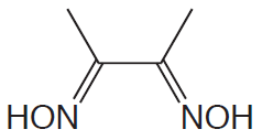Ni(C₄H₇O₂N₂)₂	Ni(C₄H₇O₂N₂)₂
Fe³⁺	cupferron		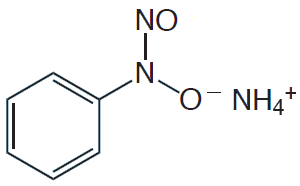Fe(C₆H₅N₂O₂)₃	Fe₂O₃
Cu²⁺	cupron		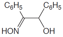CuC₁₄H₁₁O₂N	CuC₁₄H₁₁O₂N
Co²⁺	1-nitrso-2-napthol		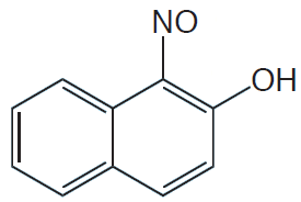Co(C₁₀H₆O₂N)₃	Co or CoSO₄
K⁺	sodium tetraphenylborate	Na[B(C₆H₅)₄]	K[B(C₆H₅)₄	K[B(C₆H₅)₄
NO₃^–	nitron		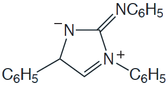C₂₀H₁₆N₄HNO₃	C₂₀H₁₆N₄HNO₃

Organic Analysis

Several organic functional groups or heteroatoms can be determined using precipitation gravimetric methods. Table \(\PageIndex{4}\) provides a summary of several representative examples. Note that the procedure for the determination of alkoxy functional groups is an indirect analysis.

**Table \(\PageIndex{4}\):** Selected Precipitation Gravimetric Methods for the Analysis of Organic Functional Groups and Heteroatoms
Analyte	Treatment	Precipitant	Precipitate
Organic halides R–X X = Cl, Br, I	Oxidation with HNO₃ in the presence of Ag⁺	AgNO₃	AgX
Organic halides R–X X = Cl, Br, I	Combustion in O₂ (with a Pt catalyst) in the presence of Ag⁺	AgNO₃	AgX
Organic sulfur	Oxidation with HNO₃ in the presence of Ba²⁺	BaCl₂	BaSO₄
Organic sulfur	Combustion in O₂ (with Pt catalyst) with SO₂ and SO₃ collected in dilute H₂O₂	BaCl₂	BaSO₄
Alkoxy groups –O–R or –COO–R R = CH₃ or C₂H₅	Reaction with HI to produce RI	AgNO₃	AgI

Quantitative Calculations

The stoichiometry of a precipitation reaction provides a mathematical relationship between the analyte and the precipitate. Because a precipitation gravimetric method may involve several chemical reactions before the precipitation reaction, knowing the stoichiometry of the precipitation reaction may not be sufficient. Even if you do not have a complete set of balanced chemical reactions, you can deduce the mathematical relationship between the analyte and the precipitate using a conservation of mass. The following example demonstrates the application of this approach to the direct analysis of a single analyte.

Example 8.1

To determine the amount of magnetite, Fe₃O₄, in an impure ore, a 1.5419-g sample is dissolved in concentrated HCl, giving a mixture of Fe²⁺ and Fe³⁺. After adding HNO₃ to oxidize Fe²⁺ to Fe³⁺ and diluting with water, Fe³⁺ is precipitated as Fe(OH)₃ by adding NH₃. Filtering, rinsing, and igniting the precipitate provides 0.8525 g of pure Fe₂O₃. Calculate the %w/w Fe₃O₄ in the sample.

Solution

A conservation of mass requires that all the iron from the ore is found in the Fe₂O₃. We know there are 2 moles of Fe per mole of Fe₂O₃ (FW = 159.69 g/mol) and 3 moles of Fe per mole of Fe₃O₄ (FW = 231.54 g/mol); thus

\[\mathrm{0.8525\;g\;Fe_2O_3\times\dfrac{2\;mol\;Fe}{159.69\;g\;Fe_2O_3}\times\dfrac{231.54\;g\;Fe_3O_4}{3\;mol\;Fe}=0.82405\;g\;Fe_3O_4}\]

The % w/w s Fe₃O₄ in the sample, therefore, is

\[\mathrm{\dfrac{0.82405\;g\;Fe_3O_4}{1.5419\;g\;sample}\times100=53.44\%\;w/w\;Fe_3O_4}\]

Exercise 8.2

A 0.7336-g sample of an alloy containing copper and zinc is dissolved in 8 M HCl and diluted to 100 mL in a volumetric flask. In one analysis, the zinc in a 25.00-mL portion of the solution is precipitated as ZnNH₄PO₄, and subsequently isolated as Zn₂P₂O₇, yielding 0.1163 g. The copper in a separate 25.00-mL portion of the solution is treated to precipitate CuSCN, yielding 0.2931 g. Calculate the %w/w Zn and the %w/w Cu in the sample.

Click here to review your answer to this exercise.

In Practice Exercise 8.2 the sample contains two analytes. Because we can selectively precipitate each analyte, finding their respective concentrations is a straightforward stoichiometric calculation. But what if we cannot precipitate the two analytes separately? To find the concentrations of both analytes, we still need to generate two precipitates, at least one of which must contain both analytes. Although this complicates the calculations, we can still use a conservation of mass to solve the problem.

Example 8.2

A 0.611-g sample of an alloy containing Al and Mg is dissolved and treated to prevent interferences by the alloy’s other constituents. Aluminum and magnesium are precipitated using 8-hydroxyquinoline, providing a mixed precipitate of Al(C₉H₆NO)₃ and Mg(C₉H₆NO)₂ that weighs 7.815 g. Igniting the precipitate converts it to a mixture of Al₂O₃ and MgO that weighs 1.002 g. Calculate the %w/w Al and %w/w Mg in the alloy.

Solution

The masses of the solids provide us with the following two Equations.

\[\mathrm{g\;Al(C_9H_6NO)_3+g\;Mg(C_9H_6NO)_2=7.815\;g}\]

\[\mathrm{g\;Al_2O_3+g\;MgO=1.002\;g}\]

With two Equations and four unknowns, we need two additional Equations to solve the problem. A conservation of mass requires that all the aluminum in Al(C₉H₆NO)₃ is found in Al₂O₃; thus

\[\mathrm{g\;Al_2O_3=g\;Al(C_9H_6NO)_3\times\dfrac{1\;mol\;Al}{459.45\;g\;Al(C_9H_6NO)_3}\times\dfrac{101.96\;g\;Al_2O_3}{2\;mol\;Al_2O_3}}\]

\[\mathrm{g\;Al_2O_3=0.11096\times g\;Al(C_9H_6NO)_3}\]

Using the same approach, a conservation of mass for magnesium gives

\[\mathrm{g\;MgO=g\;Mg(C_9H_6NO)_2\times\dfrac{1\;mol\;Mg}{312.61\;g\;Mg(C_9H_6NO)_2}\times\dfrac{40.304\;g\;MgO}{mol\;Mg}}\]

\[\mathrm{g\;MgO=0.12893\times g\;Mg(C_9H_6NO)_2}\]

Substituting the Equations for g MgO and g Al₂O₃ into the Equation for the combined weights of MgO and Al₂O₃ leaves us with two Equations and two unknowns.

\[\mathrm{g\;Al(C_9H_6NO)_3+g\;Mg(C_9H_6NO)_2=7.815\;g}\]

\[\mathrm{0.11096\times g\;Al(C_9H_6NO)_3+0.12893\times g\;Mg(C_9H_6NO)_2=1.002\;g}\]

Multiplying the first Equation by 0.11096 and subtracting the second Equation gives

\[\mathrm{-0.01797\times g\;Mg(C_9H_6NO)_2=-0.1348\;g}\]

\[\mathrm{g\;Mg(C_9H_6NO)_2=7.501\;g}\]

\[\mathrm{g\;Al(C_9H_6NO)_3=7.815\;g-7.501\;g\;Mg(C_9H_6NO)_2=0.314\;g}\]

Now we can finish the problem using the approach from Example 8.1. A conservation of mass requires that all the aluminum and magnesium in the sample of Dow metal is found in the precipitates of Al(C₉H₆NO)₃ and the Mg(C₉H₆NO)₂. For aluminum, we find that

\[\mathrm{0.314\;g\;Al(C_9H_6NO)_3\times\dfrac{1\;mol\;Al}{459.45\;g\;Al(C_9H_6NO)_3}\times\dfrac{26.982\;g\;Al}{mol\;Al}=0.01844\;g\;Al}\]

\[\mathrm{\dfrac{0.01844\;g\;Al}{0.611\;g\;sample}\times100=3.02\%\;w/w\;Al}\]

and for magnesium we have

\[\mathrm{7.501\;g\;Mg(C_9H_6NO)_2\times\dfrac{1\;mol\;Mg}{312.61\;g\;Mg(C_9H_6NO)_2}\times\dfrac{24.305\;g\;Mg}{mol\;Mg}=0.5832\;g\;Mg}\]

\[\mathrm{\dfrac{0.5832\;g\;Mg}{0.611\;g\;sample}\times100=95.5\%\;w/w\;Mg}\]

Exercise 8.3

A sample of a silicate rock weighing 0.8143 g is brought into solution and treated to yield a 0.2692-g mixture of NaCl and KCl. The mixture of chloride salts is subsequently dissolved in a mixture of ethanol and water, and treated with HClO₄, precipitating 0.5713 g of KClO₄. What is the %w/w Na₂O in the silicate rock?

Click here to review your answer to this exercise.

The previous problems are examples of direct methods of analysis because the precipitate contains the analyte. In an indirect analysis the precipitate forms as a result of a reaction with the analyte, but the analyte is not part of the precipitate. As shown by the following example, despite the additional complexity, we can use conservation principles to organize our calculations.

Example 8.3

An impure sample of Na₃PO₃ weighing 0.1392 g is dissolved in 25 mL of water. A solution containing 50 mL of 3% w/v HgCl₂, 20 mL of 10% w/v sodium acetate, and 5 mL of glacial acetic acid is then prepared. Adding the solution of Na₃PO₃ to the solution containing HgCl₂, oxidizes PO₃^3– to PO₄^3–, precipitating Hg₂Cl₂. After digesting, filtering, and rinsing the precipitate, 0.4320 g of Hg₂Cl₂ is obtained. Report the purity of the original sample as % w/w Na₃PO₃.

Solution

This is an example of an indirect analysis because the precipitate, Hg₂Cl₂, does not contain the analyte, Na₃PO₃. Although the stoichiometry of the reaction between Na₃PO₃ and HgCl₂ is given earlier in the chapter, let’s see how we can solve the problem using conservation principles.

The reaction between Na₃PO₃ and HgCl₂ is a redox reaction in which phosphorous increases its oxidation state from +3 in Na₃PO₃ to +5 in Na₃PO₄, and in which mercury decreases its oxidation state from +2 in HgCl₂ to +1 in Hg₂Cl₂. A redox reaction must obey a conservation of electrons—all the electrons released by the reducing agent, Na₃PO₃, must be accepted by the oxidizing agent, HgCl₂. Knowing this, we write the following stoichiometric conversion factors:

\[\dfrac{2\;\mathrm{mol}\;e^-}{\mathrm{mol\;Na_3PO_4}}\textrm{ and }\dfrac{1\;\mathrm{mol}\;e^-}{\mathrm{mol\;HgCl_2}}\]

(Although you can write the balanced reactions for any analysis, applying conservation principles can save you a significant amount of time!)

Now we are ready to solve the problem. First, we use a conservation of mass for mercury to convert the precipitate’s mass to the moles of HgCl₂.

\[\mathrm{0.4320\;g\;Hg_2Cl_2\times\dfrac{2\;mol\;Hg}{472.09\;g\;HgCl}\times\dfrac{1\;mol\;HgCl_2}{mol\;Hg}=1.8302\times10^{-3}\;mol\;HgCl_2}\]

Next, we use the conservation of electrons to find the mass of Na₃PO₃.

\[\mathrm{1.8302\times10^{-3}\;mol\;HgCl_2}\times\dfrac{\mathrm{1\;mol}\;e^-}{\mathrm{mol\;HgCl_2}}\times\dfrac{\mathrm{1\;mol\;Na_3PO_3}}{\mathrm{2\;mol}\;e^-}\times\mathrm{\dfrac{147.94\;g\;Na_3PO_3}{mol\;Na_3PO_3}=0.13538\;g\;Na_3PO_3}\]

(As you become comfortable with using conservation principles, you will see opportunities for further simplifying problems. For example, a conservation of electrons requires that the electrons released by Na₃PO₃ end up in the product, Hg₂Cl₂, yielding the following stoichiometric conversion factor:

\[\dfrac{\mathrm{2\;mol}\;e^-}{\mathrm{mol\;Hg_2Cl_2}}\]

This conversion factor provides a direct link between the mass of Hg₂Cl₂ and the mass of Na₃PO₃.)

Finally, we calculate the %w/w Na₃PO₃ in the sample.

\[\mathrm{\dfrac{0.13538\;g\;Na_3PO_3}{0.1392\;g\;sample}\times100=97.26\%\;w/w\;Na_3PO_3}\]

Practice Exercise 8.4

One approach for determining phosphate, PO₄^3–, is to precipitate it as ammonium phosphomolybdate, (NH₄)₃PO₄•12MoO₃. After isolating the precipitate by filtration, it is dissolved in acid and the molybdate precipitated and weighed as PbMoO₃. Suppose we know that our samples contain at least 12.5% Na₃PO₄ and we need to recover a minimum of 0.600 g of PbMoO₃? What is the minimum amount of sample needed for each analysis?

Click here to review your answer to this exercise.

8.2.2 Qualitative Applications

A precipitation reaction is a useful method for identifying inorganic and organic analytes. Because a qualitative analysis does not require quantitative measurements, the analytical signal is simply the observation that a precipitate has formed. Although qualitative applications of precipitation gravimetry have been largely replaced by spectroscopic methods of analysis, they continue to find application in spot testing for the presence of specific analytes.⁹

Note

Any of the precipitants listed in Table \(\PageIndex{1}\), Table \(\PageIndex{3}\), and Table \(\PageIndex{4}\) can be used for a qualitative analysis.

8.2.3 Evaluating Precipitation Gravimetry

Scale of Operation

The scale of operation for precipitation gravimetry is limited by the sensitivity of the balance and the availability of sample. To achieve an accuracy of ±0.1% using an analytical balance with a sensitivity of ±0.1 mg, we must isolate at least 100 mg of precipitate. As a consequence, precipitation gravimetry is usually limited to major or minor analytes, in macro or meso samples (see Figure 3.5 in Chapter 3). The analysis of trace level analytes or micro samples usually requires a microanalytical balance.

Accuracy

For a macro sample containing a major analyte, a relative error of 0.1–0.2% is routinely achieved. The principle limitations are solubility losses, impurities in the precipitate, and the loss of precipitate during handling. When it is difficult to obtain a precipitate that is free from impurities, it may be possible to determine an empirical relationship between the precipitate’s mass and the mass of the analyte by an appropriate calibration.

Note

Problem 8.27 provides an example of how to determine an analyte’s concentration by establishing an empirical relationship between the analyte and the precipitate.

Precision

The relative precision of precipitation gravimetry depends on the sample’s size and the precipitate’s mass. For a smaller amount of sample or precipitate, a relative precision of 1–2 ppt is routinely obtained. When working with larger amounts of sample or precipitate, the relative precision can be extended to several ppm. Few quantitative techniques can achieve this level of precision.

Sensitivity

For any precipitation gravimetric method we can write the following general Equation relating the signal (grams of precipitate) to the absolute amount of analyte in the sample

\[\textrm{grams precipitate}=k\times\textrm{grams analyte}\label{8.13}\]

Note

Equation 8.13 assumes that we have used a suitable blank to correct the signal for any contributions of the reagent to the precipitate’s mass.

where k, the method’s sensitivity, is determined by the stoichiometry between the precipitate and the analyte. Consider, for example, the determination of Fe as Fe₂O₃. Using a conservation of mass for iron, the precipitate’s mass is

\[\mathrm{g\;Fe_2O_3=g\;Fe\times\dfrac{1\;mol\;Fe}{AW\;Fe}\times\dfrac{FW\;Fe_2O_3}{2\;mol\;Fe}}\]

and the value of k is

\[k=\dfrac{1}{2}\times\mathrm{\dfrac{FW\;Fe_2O_3}{AW\;Fe}}\label{8.14}\]

As we can see from Equation 8.14, there are two ways to improve a method’s sensitivity. The most obvious way to improve sensitivity is to increase the ratio of the precipitate’s molar mass to that of the analyte. In other words, it helps to form a precipitate with the largest possible formula weight. A less obvious way to improve a method’s sensitivity is indicated by the term of 1/2 in Equation 8.14, which accounts for the stoichiometry between the analyte and precipitate. We can also improve sensitivity by forming a precipitate that contains fewer units of the analyte.

Exercise 8.5

Suppose you wish to determine the amount of iron in a sample. Which of the following compounds—FeO, Fe₂O₃, or Fe₃O₄—provides the greatest sensitivity?

Click here to review your answer to this exercise.

Selectivity

Due to the chemical nature of the precipitation process, precipitants are usually not selective for a single analyte. For example, silver is not a selective precipitant for chloride because it also forms precipitates with bromide and iodide. Interferents are often a serious problem and must be considered if accurate results are to be obtained.

Time, Cost, and Equipment

Precipitation gravimetry is time intensive and rarely practical if you have a large number of samples to analyze. However, because much of the time invested in precipitation gravimetry does not require an analyst’s immediate supervision, it may be a practical alternative when working with only a few samples. Equipment needs are few—beakers, filtering devices, ovens or burners, and balances—inexpensive, routinely available in most laboratories, and easy to maintain.

Contributors

David Harvey (DePauw University)