
14.3: Validating the Method as a Standard Method
- Page ID
- 5583

For an analytical method to be useful, an analyst must be able to achieve results of acceptable accuracy and precision. Verifying a method, as described in the previous section, establishes this goal for a single analyst. Another requirement for a useful analytical method is that an analyst should obtain the same result from day to day, and different labs should obtain the same result when analyzing the same sample. The process by which we approve method for general use is known as validation and it involves a collaborative test of the method by analysts in several laboratories. Collaborative testing is used routinely by regulatory agencies and professional organizations, such as the U. S. Environmental Protection Agency, the American Society for Testing and Materials, the Association of Official Analytical Chemists, and the American Public Health Association. Many of the representative methods in earlier chapters are identified by these agencies as validated methods.
Representative Method 10.1 for the determination of iron in water and wastewater, and Representative Method 10.5 for the determination of sulfate in water, are two examples of standard methods validated through collaborative testing.
When an analyst performs a single analysis on a sample the difference between the experimentally determined value and the expected value is influenced by three sources of error: random errors, systematic errors inherent to the method, and systematic errors unique to the analyst. If the analyst performs enough replicate analyses, then we can plot a distribution of results, as shown in Figure 14.18a. The width of this distribution is described by a standard deviation, providing an estimate of the random errors effecting the analysis. The position of the distribution’s mean, X, relative to the sample’s true value, μ, is determined both by systematic errors inherent to the method and those systematic errors unique to the analyst. For a single analyst there is no way to separate the total systematic error into its component parts.
The goal of a collaborative test is to determine the magnitude of all three sources of error. If several analysts each analyze the same sample one time, the variation in their collective results, as shown in Figure 14.18b, includes contributions from random errors and those systematic errors (biases) unique to the analysts. Without additional information, we cannot separate the standard deviation for this pooled data into the precision of the analysis and the systematic errors introduced by the analysts. We can use the position of the distribution, to detect the presence of a systematic error in the method.
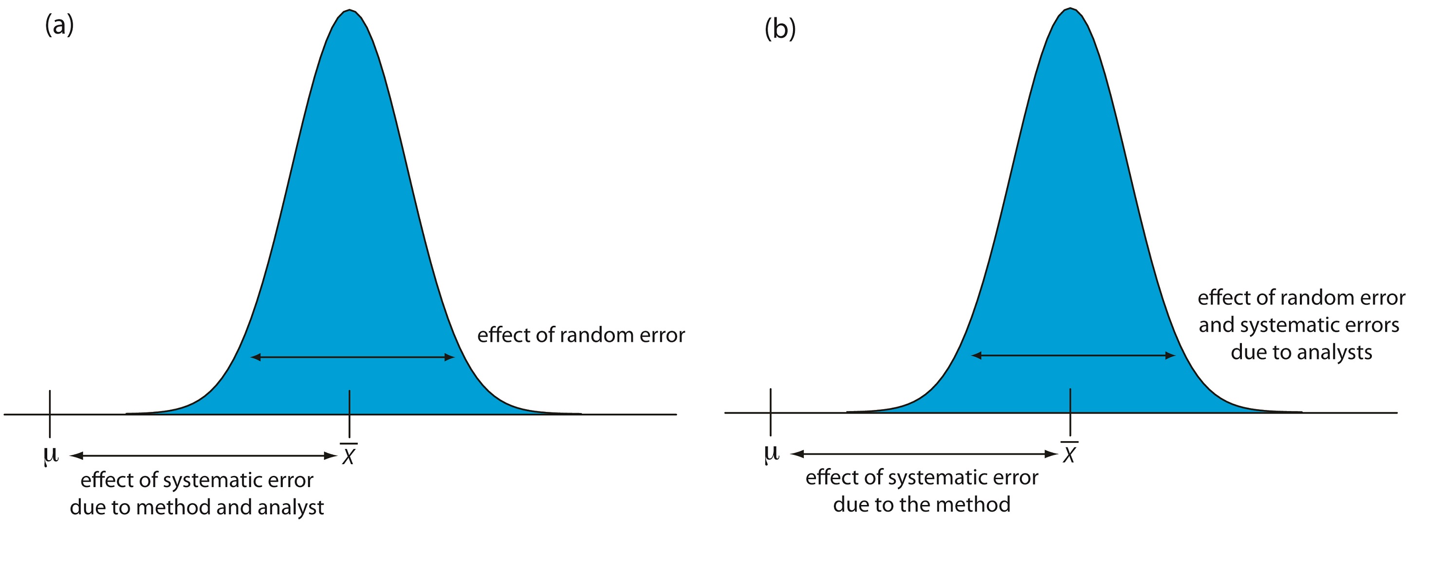
Figure 14.18 Partitioning of random errors, systematic errors due to the analyst, and systematic errors due to the method for (a) replicate analyses performed by a single analyst, and (b) single determinations performed by several analysts.
14.3.1 Two-Sample Collaborative Testing
The design of a collaborative test must provide the additional information we need to separate random errors from the systematic errors introduced by the analysts. One simple approach—accepted by the Association of Official Analytical Chemists—is to have each analyst analyze two samples that are similar in both their matrix and in their concentration of analyte. To analyze their results we represent each analyst as a single point on a two-sample chart, using the result for one sample as the x-coordinate and the result for the other sample as the y-coordinate.8
As shown in Figure 14.19, a two-sample chart divides the results into four quadrants, which we identify as (+, +), (–, +), (–, –) and (+, –), where a plus sign indicates that the analyst’s result exceeds the mean for all analysts and a minus sign indicates that the analyst’s result is smaller than the mean for all analysts. The quadrant (+, –), for example, contains results for analysts that exceeded the mean for sample X and that undershot the mean for sample Y. If the variation in results is dominated by random errors, then we expect the points to be distributed randomly in all four quadrants, with an equal number of points in each quadrant. Furthermore, as shown in Figure 14.19a, the points will cluster in a circular pattern whose center is the mean values for the two samples. When systematic errors are significantly larger than random errors, then the points occur primarily in the (+, +) and the (–, –) quadrants, forming an elliptical pattern around a line bisecting these quadrants at a 45o angle, as seen in Figure 14.19b.
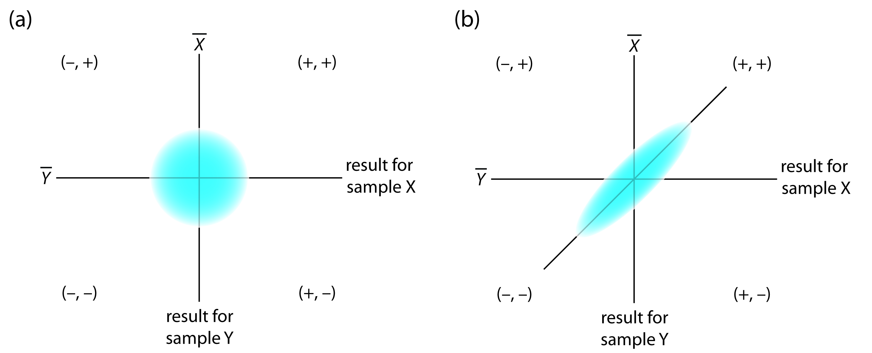
Figure 14.19 Typical two-sample plots when (a) random errors are significantly larger than systematic errors due to the analysts, and (b) when systematic errors due to the analysts are significantly larger than the random errors.
A visual inspection of a two-sample chart is an effective method for qualitatively evaluating the results of analysts and the capabilities of a proposed standard method. If random errors are insignificant, then the points fall on the 45o line. The length of a perpendicular line from any point to the 45o line, therefore, is proportional to the effect of random error on that analyst’s results. The distance from the intersection of the axes—corresponding to the mean values for samples X and Y—to the perpendicular projection of a point on the 45o line is proportional to the analyst’s systematic error. Figure 14.20 illustrates these relationships. An ideal standard method has small random errors and small systematic errors due to the analysts, and has a compact clustering of points that is more circular than elliptical.
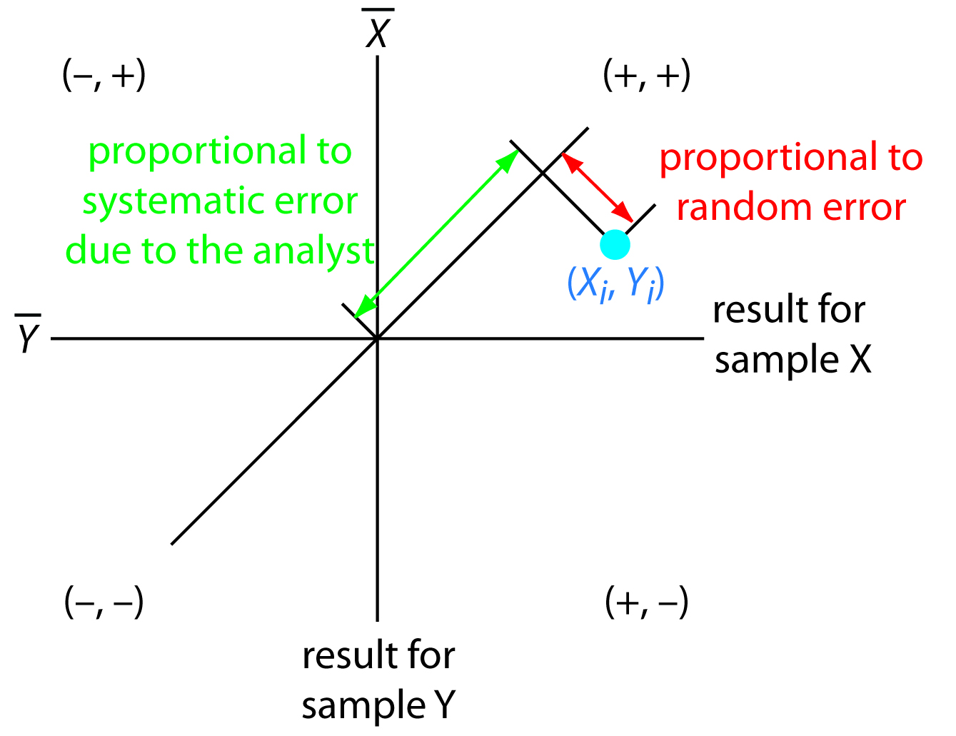
Figure 14.20 Relationship between the result for a single analyst (in blue) and the contribution of random error (red arrow) and the contribution from the analyst’s systematic error (green arrow).
We also can use the data in a two-sample chart to separate the total variation in the data, σtot, into contributions from random error, σrand, and systematic errors due to the analysts, σsyst.9 Because an analyst’s systematic errors are present in his or her analysis of both samples, the difference, D, between the results
\[D_i = X_i - Y_i\]
is the result of random error. To estimate the total contribution from random error we use the standard deviation of these differences, sD, for all analysts
\[s_\textrm D=\sqrt{\dfrac{\sum (D_i-\overline D)^2}{2(n-1)}}=s_{\textrm{rand}}\approx \sigma_{\textrm{rand}}\tag{14.18}\]
where n is the number of analysts. The factor of 2 in the denominator of equation 14.18 is the result of using two values to determine Di. The total, T, of each analyst’s results
\[T_i = X_i + Y_i\]
contains contributions from both random error and twice the analyst’s systematic error.
\[\sigma_{\textrm{tot}}^2=\sigma_{\textrm{rand}}^2+2\sigma_{\textrm{syst}}^2\tag{14.19}\]
We double the analyst’s systematic error in equation 14.19 because it is the same in each analysis.
The standard deviation of the totals, sT, provides an estimate for σtot.
\[s_\textrm T=\sqrt {\dfrac{\sum (T_i-\overline T)^2}{2(n-1)}}=s_{\textrm{tot}}\approx \sigma_{\textrm{tot}}\tag{14.20}\]
Again, the factor of 2 in the denominator is the result of using two values to determine Ti.
If the systematic errors are significantly larger than the random errors, then sT is larger than sD, a hypothesis we can evaluate using a one-tailed F‑test
\[F=\dfrac{s_\textrm T^2}{s_\textrm D^2}\]
where the degrees of freedom for both the numerator and the denominator are n – 1. As shown in the following example, if sT is significantly larger than sD we can use equation 14.19 to separate σtot2 into components representing random error and systematic error.
For a review of the F-test, see Section 4.6.2 and Section 4.6.3. Example 4.18 illustrates a typical application.
Example 14.6
As part of a collaborative study of a new method for determining the amount of total cholesterol in blood, you send two samples to 10 analysts with instructions to analyze each sample one time. The following results, in mg total cholesterol per 100 mL of serum, are returned to you.
| analyst | sample 1 | sample 2 |
|---|---|---|
| 1 | 245.0 | 229.4 |
| 2 | 247.4 | 249.7 |
| 3 | 246.0 | 240.4 |
| 4 | 244.9 | 235.5 |
| 5 | 255.7 | 261.7 |
| 6 | 248.0 | 239.4 |
| 7 | 249.2 | 255.5 |
| 8 | 255.1 | 224.3 |
| 9 | 255.0 | 246.3 |
| 10 | 243.1 | 253.1 |
Use this data estimate σrand and σsyst for the method.
Solution
Figure 14.21 provides a two-sample plot of the results. The clustering of points suggests that the systematic errors of the analysts are significant. The vertical line at 245.9 mg/100 mL is the average value for sample 1 and the average value for sample 2 is shown by the horizontal line at 243.5 mg/100 mL. To estimate σrand and σsyst we first calculate values for Di and Ti.
| analyst | Di | Ti |
|---|---|---|
| 1 | 15.6 | 474.4 |
| 2 | -2.3 | 497.1 |
| 3 | 5.6 | 486.4 |
| 4 | 9.4 | 480.4 |
| 5 | -6.0 | 517.4 |
| 6 | 8.6 | 487.4 |
| 7 | -6.3 | 504.7 |
| 8 | 0.8 | 449.4 |
| 9 | 8.7 | 501.3 |
| 10 | -10.0 | 496.2 |
Next, we calculate the standard deviations for the differences, sD, and the totals, sT, using equations 14.18 and 14.20, giving sD = 5.95 and sT = 13.3. To determine if the systematic errors between the analysts are significant, we use an F-test to compare sT and sD.
\[F=\dfrac{s_\textrm T^2}{s_\textrm D^2}=\dfrac{(13.3)^2}{(5.95)^2}=5.00\]
Because the F-ratio is larger than F(0.05, 9, 9), which is 3.179, we conclude that the systematic errors between the analysts are significant at the 95% confidence level. The estimated precision for a single analyst is
\[\sigma_{\textrm{rand}}\approx s_\textrm D=5.95\]
(Critical values for the F-test are in Appendix 5.)
The estimated standard deviation due to systematic errors between analysts is calculated from equation 14.18.
\[\sigma_{\textrm{syst}}\approx \sqrt{\dfrac{\sigma_{\textrm{tot}}^2-\sigma_{\textrm{rand}}^2}{2}}\approx \sqrt{\dfrac{s_\textrm T^2-s_\textrm D^2}{2}}=\sqrt{\dfrac{(13.3)^2-(5.95)^2}{2}}=8.41\]
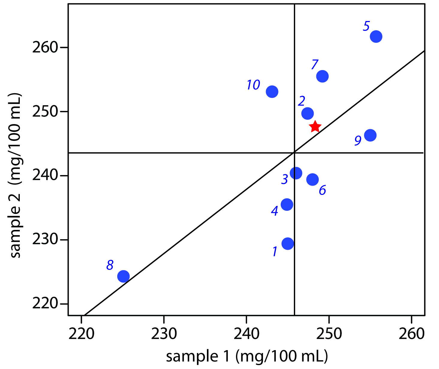
Figure 14.21 Two-sample plot for the data in Example 14.6. The number by each blue point indicates the analyst. The true values for each sample (see Example 14.7) are indicated by the red star.
If the true values for the two samples are known, we also can test for the presence of a systematic error in the method. If there are no systematic method errors, then the sum of the true values, μtot, for samples X and Y
\[\mu_\ce{tot} = \mu_\ce{X} + \mu_\ce{Y}\]
should fall within the confidence interval around T. We can use a two-tailed t-test of the following null and alternate hypotheses
\[H_0:\overline{T}= \mu_\ce{tot} \hspace{30px} H_\ce{A}: \overline{T}≠ \mu_\ce{tot}\]
to determine if there is evidence for a systematic error in the method. The test statistic, texp, is
\[t_{\textrm{exp}}=\dfrac{|\overline T-\,\mu_{\textrm{tot}}|\sqrt n}{s_\textrm T\sqrt2}\tag{14.21}\]
with n – 1 degrees of freedom. We include the √2 in the denominator because sT (see equation 14.20) underestimates the standard deviation when comparing T to μtot.
For a review of the t-test of an experimental mean to a known mean, see Section 4.6.1. Example 4.16 illustrates a typical application.
Example 14.7
The two samples analyzed in Example 14.6 are known to contain the following concentrations of cholesterol
\[\mathrm{\mu_{samp\: 1} = 248.3\: mg/100\: mL \hspace{30px} \mu_{samp\: 2} = 247.6\: mg/100\: mL}\]
Determine if there is any evidence for a systematic error in the method at the 95% confidence level.
Solution
Using the data from Example 14.6 and the true values for the samples, we know that sT is 13.3, and that
\[\overline{T} = \overline{X}_\textrm{samp 1} + \overline{X}_\textrm{samp 2} = 245.9 + 243.5 = \textrm{489.4 mg/100 mL}\]
\[\mu_\textrm{tot} = \mu_\textrm{samp 1} + \mu_\textrm{samp 2} = 248.3 + 247.6 = \textrm{495.9 mg/100 mL}\]
Substituting these values into equation 14.21 gives
\[t_{\textrm{exp}}=\dfrac{|489.4-495.9|\sqrt{10}}{13.3\sqrt2}=1.09\]
Because this value for texp is smaller than the critical value of 2.26 for t(0.05, 9), there is no evidence for a systematic error in the method at the 95% confidence level.
(Critical values for the t-test are in Appendix 4.)
Example 14.6 and Example 14.7 illustrate how we can use a pair of similar samples in a collaborative test of a new method. Ideally, a collaborative test involves several pairs of samples that span the range of analyte concentrations for which we plan to use the method. In doing so, we evaluate the method for constant sources of error and establish the expected relative standard deviation and bias for different levels of analyte.
14.3.2 Collaborative Testing and Analysis of Variance
In a two-sample collaborative test we ask each analyst to perform a single determination on each of two separate samples. After reducing the data to a set of differences, D, and a set of totals, T, each characterized by a mean and a standard deviation, we extract values for the random errors affecting precision and the systematic differences between then analysts. The calculations are relatively simple and straightforward.
An alternative approach for completing a collaborative test is to have each analyst perform several replicate determinations on a single, common sample. This approach generates a separate data set for each analyst, requiring a different statistical treatment to arrive at estimates for σrand and σsyst.
There are several statistical methods for comparing three or more sets of data. The approach we consider in this section is an analysis of variance (ANOVA). In its simplest form, a one-way ANOVA allows us to explore the importance of a single variable—the identity of the analyst is one example—on the total variance. To evaluate the importance of this variable, we compare its variance to the variance explained by indeterminate sources of error.
We first introduced variance in Chapter 4 as one measure of a data set’s spread around its central tendency. In the context of an analysis of variance, it is useful for us to understand that variance is simply a ratio of two terms: a sum of squares for the differences between individual values and their mean, and the available degrees of freedom. For example, the variance, s2, of a data set consisting of n measurements is
\[s^2=\dfrac{\sum (X_i-\overline X)^2}{n-1}=\dfrac{\textrm{sum of squares}}{\textrm{degrees of freedom}}\]
where Xi is the value of a single measurement and X is the mean. The ability to partition the variance into a sum of squares and the degrees of freedom greatly simplifies the calculations in a one-way ANOVA.
Let’s use a simple example to develop the rationale behind a one-way ANOVA calculation. The data in Table 14.6 are from four analysts, each asked to determine the purity of a single pharmaceutical preparation of sulfanilamide. Each column in Table 14.6 provides the results for an individual analyst. To help us keep track of this data, we will represent each result as Xij, where i identifies the analyst and j indicates the replicate. For example, X3,5 is the fifth replicate for the third analyst, or 94.24%.
| replicate | analyst A | analyst B | analyst C | analyst D |
|---|---|---|---|---|
| 1 | 94.09 | 99.55 | 95.14 | 93.88 |
| 2 | 94.64 | 98.24 | 94.62 | 94.23 |
| 3 | 95.08 | 101.1 | 95.28 | 96.05 |
| 4 | 94.54 | 100.4 | 94.59 | 93.89 |
| 5 | 95.38 | 100.1 | 94.24 | 94.95 |
| 6 | 93.62 | 95.49 | ||
| X | 94.56 | 99.88 | 95.86 | 94.77 |
| s | 0.630 | 1.073 | 0.428 | 0.899 |
The data in Table 14.6 show variability, both in the results obtained by each analyst and in the difference in the results between the analysts. There are two sources for this variability: indeterminate errors associated with the analytical procedure experienced equally by each analyst, and systematic or determinate errors introduced by individual analysts.
One way to view the data in Table 14.6 is to treat it as a single large sample, characterized by a global mean and a global variance
\[\overline{\overline X}=\dfrac{\sum_{i=1}^{h}\sum_{j=1}^{n_i}X_{ij}}{N}\tag{14.22}\]
where h is the total number of samples (in this case the number of analysts), ni is the number of replicates for the ith sample (in this case the ith analyst), and N is the total number of data points (in this case 22). The global variance—which includes all sources of variability affecting the data—provides an estimate of the combined influence of indeterminate errors and systematic errors.
A second way to work with the data in Table 14.6 is to treat the results for each analyst separately. If we assume that each analyst experiences the same indeterminate errors, then the variance, s2, for each analyst provides a separate estimate of σrand2. To pool these individual variances, which we call the within-sample variance, sw2, we square the difference between each replicate and its corresponding mean, add them up, and divide by the degrees of freedom.
\[\sigma _{\textrm{rand}}^2\approx s_\textrm w^2=\dfrac{\sum_{i=1}^{h}\sum_{j=1}^{n_i}( X_{ij}-\overline X_i)^2}{N-h}\tag{14.24}\]
Note
Carefully compare our description of equation 14.24 to the equation itself. It is important that you understand why equation 14.24 provides our best estimate of the indeterminate errors affecting the data in Table 14.6. Note that we lose one degree of freedom for each of the h means included in the calculation.
Equation 14.24 provides an estimate for σrand2. To estimate the systematic errors, σsyst2, affecting the results in Table 14.6 we need to consider the differences between the analysts. The variance of the individual mean values about the global mean, which we call the between-sample variance, sb2, provides this estimate.
\[\sigma _{\textrm{syst}}^2\approx s_\textrm b^2=\dfrac{\sum_{i=1}^{h}n_i(\overline X_i-\overline{\overline{X}})^2}{h-1}\tag{14.25}\]
Note
We lose one degree of freedom for the global mean.
The between-sample variance includes contributions from both indeterminate errors and systematic errors
\[s_\ce{b}^2= σ_\ce{rand}^2 + \bar{n}σ_\ce{syst}^2\tag{14.26}\]
where n is the average number of replicates per analyst.
\[\bar n = \dfrac{\sum_{i=1}^{h}n_i}{h}\]
Note
Note the similarity between equation 14.26 and equation 14.19. The analysis of the data in a two-sample plot is the same as a one-way analysis of variance with h = 2.
In a one-way ANOVA of the data in Table 14.6 we make the null hypothesis that there are no significant differences between the mean values for each analyst. The alternative hypothesis is that at least one of the means is significantly different. If the null hypothesis is true, then σsyst2 must be zero, and sw2 and sb2 should have similar values. If sb2 is significantly greater than sw2, then σsyst2 is greater than zero. In this case we must accept the alternative hypothesis that there is a significant difference between the means for the analysts. The test statistic is the F-ratio
\[F_{\textrm{exp}}=\dfrac{s_\ce{b}^2}{s_\ce{w}^2}\]
which is compared to the critical value F(α, h – 1, N – h). This is a one-tailed significance test because we are only interested in whether sb2 is significantly greater than sw2.
Both sb2 and sw2 are easy to calculate for small data sets. For larger data sets, calculating sw2 is tedious. We can simplify the calculations by taking advantage of the relationship between the sum-of-squares terms for the global variance (equation 14.23), the within-sample variance (equation 14.24), and the between-sample variance (equation 14.25). We can split the numerator of equation 14.23, which is the total sum-of-squares, SSt, into two terms
\[SS_\ce{t} = SS_\ce{w} + SS_\ce{b}\]
where SSw is the sum-of-squares for the within-sample variance and SSb is the sum-of-squares for the between-sample variance. Calculating SSt and SSb gives SSw by difference. Finally, dividing SSw and SSb by their respective degrees of freedom gives sw2 and sb2. Table 14.7 summarizes the equations for a one-way ANOVA calculation. Example 14.8 walks you through the calculations, using the data in Table 14.6. Section 14D provides instructions on using Excel and R to complete a one-way analysis of variance.
Note
Problem 14.17 in the end of chapter problems asks you to verify this relationship between the sum-of-squares.
|
source |
sum-of-squares |
degrees of |
variance |
expected variance |
F-ratio |
|---|---|---|---|---|---|
| between samples |
\(SS_\textrm b = \sum_{i=1}^{h}n_i(\overline X_i-\overline{\overline{X}})^2\) |
\(h - 1\) |
\(s_\textrm b^2=\dfrac{SS_\textrm b}{h-1}\) |
\(s_\textrm b^2=\sigma _{\textrm{rand}}^2+\bar n\sigma_{\textrm{syst}}^2\) |
\(F_{\textrm{exp}}=\dfrac{s_\textrm b^2}{s_\textrm w^2}\) |
| within samples |
\(SS_\ce{t} = SS_\ce{w} + SS_\ce{b}\) |
\(N - h\) |
\(s_\textrm w^2=\dfrac{SS_\textrm w}{N-h}\) |
\(s_\ce{w}^2 = σ_\ce{rand}^2\) |
|
| total |
\(\begin{align} |
\(N - 1\) |
|
|
|
Example 14.8
The data in Table 14.6 are from four analysts, each asked to determine the purity of a single pharmaceutical preparation of sulfanilamide. Determine if the difference in their results is significant at α = 0.05. If such a difference exists, estimate values for σrand2 and σsyst2.
Solution
To begin we calculate the global mean (equation 14.22) and the global variance (equation 14.23) for the pooled data, and the means for each analyst; these values are summarized here.
\[\overline{\overline X}=95.87 \hspace{5 mm}\overline{\overline {s^2}}=5.506\]
\[\overline X_\textrm A=94.56 \hspace{5 mm}\overline X_\textrm B=99.88\hspace{5 mm}\overline X_\textrm C=94.77\hspace{5 mm}\overline X_\textrm S=94.75\]
Using these values we calculate the total sum of squares
\[SS_\textrm t=\overline{\overline{s^2}}(N-1)=(5.506)(22-1)\]
the between sample sum of squares
\[SS_\textrm b=\sum_{i=1}^{h}n_i(\overline X_i-\overline{\overline X})=6(94.56-95.87)^2+5(99.88-95.87)^2 +5(94.77-95.87)^2+6(94.75-95.87)^2=104.27\]
and the within sample sum of squares
\[SS_\ce{w} = SS_\ce{t} - SS_\ce{b} = 115.63 - 104.27 = 11.36\]
The remainder of the necessary calculations are summarized in the following table.
|
source |
sum-of-squares |
degrees of freedom |
variance |
|---|---|---|---|
|
between samples |
104.27 |
h – 1 = 4 – 1 = 3 |
34.76 |
|
within samples |
11.36 |
N – h = 22 – 4 = 8 |
0.631 |
Comparing the variances we find that
\[F_{\textrm{exp}}=\dfrac{s_\textrm b^2}{s_\textrm w^2}=\dfrac{34.76}{0.631}=55.08\]
Because Fexp is greater than F(0.05, 3, 18), which is 3.16, we reject the null hypothesis and accept the alternative hypothesis that the work of at least one analyst is significantly different from the remaining analysts. Our best estimate of the within sample variance is
\[\sigma_{\textrm{rand}}^2\approx s_\textrm w^2=0.631\]
and our best estimate of the between sample variance is
\[\sigma_{\textrm{syst}}^2\approx \dfrac{s_\textrm b^2-s_\textrm w^2}{\bar n}=\dfrac {34.76-0.631}{22/4}=6.205\]
In this example the variance due to systematic differences between the analysts is almost an order of magnitude greater than the variance due to the method’s precision.
Having demonstrated that there is significant difference between the analysts, we can use a modified version of the t-test, known as Fisher’s least significant difference, to determine which analyst or analysts are responsible for the difference. The test statistic for comparing two mean values is the t-test given in equation 4.21 in Chapter 4, except we replace the pooled standard deviation, spool, by the square root of the within-sample variance from the analysis of variance.
\[t_{\textrm{exp}}=\dfrac{|\overline X_1-\overline X_2|}{\sqrt {s_\textrm w^2}\sqrt{\dfrac{1}{n_\textrm A}+\dfrac{1}{n_\textrm B}}}=\dfrac{|\overline X_1-\overline X_2|}{\sqrt{s_\textrm w^2}}\times \sqrt{\dfrac{n_\textrm An_\textrm B}{n_\textrm A+n_\textrm B}}\tag{14.27}\]
We compare texp to its critical value t(α, ν) using the same significance level as the ANOVA calculation. The degrees of freedom are the same as that for the within sample variance. Since we are interested in whether the larger of the two means is significantly greater than the other mean, the value of t(α, ν) is that for a one-tailed significance test.
You might ask why we bother with the analysis of variance if we are planning to use a t-test to compare pairs of analysts. Each t-test carries a probability, α, of claiming that a difference is significant even though it is not (a type 1 error). If we set α to 0.05 and complete six t-tests, the probability of a type 1 error increases to 0.265. Knowing that there is a significant difference within a data set—what we gain from the analysis of variance—protects the t-test.
Example 14.9
In Example 14.8 we showed that there is a significant difference between the work of the four analysts in Table 14.6. Determine the source of this significant difference.
Solution
Individual comparisons using Fisher’s least significant difference test are based on the following null hypothesis and the appropriate one-tailed alternative hypothesis.
\[H_0: \overline{X}_i =\overline{X}_j \hspace{30px} H_\ce{A}:\textrm{ one of the following }\overline{X}_i > \overline{X}_j\textrm{ or }\overline{X}_i < \overline{X}_j\]
Using equation 14.27 we calculate values of texp for each possible comparison and compare them to the one-tailed critical value of 1.73 for t(0.05, 18). For example, texp for analysts A and B is
\[ (t_{\textrm{exp}})_{\textrm{A,B}}=\dfrac{|\overline X_1-\overline X_2|}{\sqrt{s_\textrm w^2}}\times \sqrt{\dfrac{n_\textrm An_\textrm B}{n_\textrm A+n_\textrm B}}=\dfrac{|94.56-99.88|}{\sqrt{0.631}}\times \sqrt{\dfrac{6 \times 5}{6+5}}=11.06\]
Because (texp)A,B is greater than t(0.05, 18) we reject the null hypothesis and accept the alternative hypothesis that the results for analyst B are significantly greater than those for analyst A. Continuing with the other pairs it is easy to show that (texp)A,C is 0.437, (texp)A,D is 0.414, (texp)B,C is 10.17, (texp)B,D is 10.67, and (texp)C,D is 0.04. Collectively, these results suggest that there is a significant systematic difference between the work of analyst B and the work of the other analysts. There is no way to decide whether any of the four analysts has done accurate work.
(We know that analyst B’s result is significantly different than the results for analysts A, C, and D, and that we have no evidence that there is any significant difference between the results of analysts A, C, and D. We do not know if analyst B’s results is accurate, or if the results of analysts A, C, and D are accurate. In fact, it is possible that none of the results in Table 14.6 are accurate.)
We can extend an analysis of variance to systems involving more than a single variable. For example, we can use a two-way ANOVA to determine the effect on an analytical method of both the analyst and the instrumentation. The treatment of multivariate ANOVA is beyond the scope of this text, but is covered in several of the texts listed in this chapter’s additional resources.
14.3.3 What is a Reasonable Result for a Collaborative Study?
Collaborative testing provides us with a method for estimating the variability (or reproducibility) between analysts in different labs. If the variability is significant, we can determine what portion is due to indeterminate method errors (σrand2) and what portion is due to systematic differences between the analysts (σsyst2). What we have left unanswered is the following important question: What is a reasonable value for a method’s reproducibility?
An analysis of nearly 10 000 collaborative studies suggests that a reasonable estimate for a method’s reproducibility is
\[R=2^{(1-0.5\log C)}\tag{14.28}\]
where R is the percent relative standard deviation for the results included in the collaborative study and C is the fractional amount of analyte in the sample on a weight-to-weight basis.10 Equation 14.28 appears to be independent of the type of analyte, the type of matrix, and the method of analysis. For example, when a sample in a collaborative study contains 1 microgram of analyte per gram of sample, C is 10–6 and the estimated relative standard deviation is
\[R=2^{(1-0.5\log 10^{-6})}=16\%\]
For a discussion of the limitations of equation 14.28, see Linsinger, T. P. J.; Josephs, R. D. “Limitations of the Application of the Horwitz Equation,” Trends Anal. Chem. 2006, 25, 1125–1130, as well as a rebuttal (Thompson, M. “Limitations of the Application of the Horwitz Equation: A Rebuttal,” Trends Anal. Chem. 2007, 26, 659–661) and response (Linsinger, T. P. J.; Josephs, R. D. “Reply to Professor Michael Thompson’s Rebuttal,” Trends Anal. Chem. 2007, 26, 662–663.
Example 14.10
What is the estimated relative standard deviation for the results of a collaborative study when the sample is pure analyte (100% w/w analyte)? Repeat for the case where the analyte’s concentration is 0.1% w/w.
Solution
When the sample is 100% w/w analyte (C = 1) the estimated relative standard deviation is
\[R=2^{(1-0.5\log 1)}=2\%\]
We expect that approximately 67% of the participants in the collaborative study (±1σ) will report the analyte’s concentration within the range of 98% w/w to 102% w/w. If the analyte’s concentration is 0.1% w/w (C = 0.001), the estimated relative standard deviation is
\[R=2^{(1-0.5\log 0.001)}=5.7\%\]
and we expect that 67% of the analysts will report the analyte’s concentration within the range of 0.094% w/w to 0.106% w/w.
(For a normal distribution, 68.26% of the results fall within ±1s of the population’s mean (see Table 4.12).)
Of course, equation 14.28 only estimates the expected relative standard. If the method’s relative standard deviation falls with a range of one-half to twice the estimated value, then it is acceptable for use by analysts in different laboratories. The percent relative standard deviation for a single analyst should be one-half to two-thirds of that for the variability between analysts.