
14.4: Using Excel and R for an Analysis of Variance
- Page ID
- 5584

Although the calculations for an analysis of variance are relatively straightforward, they can be tedious for large data sets. Both Excel and R include functions for completing an analysis of variance. In addition, R provides a function for identifying the source(s) of significant differences within the data set.
14.4.1 Excel
Excel’s Analysis ToolPak includes a tool to help you complete an analysis of variance. Let’s use the ToolPak to complete an analysis of variance on the data in Table 14.6. Enter the data from Table 14.6 into a spreadsheet as shown in Figure 14.22. To complete the analysis of variance select Data Analysis... from the Tools menu, which opens a window entitled “Data Analysis.” Scroll through the window, select Analysis: Single Factor from the available options, and click OK. Place the cursor in the box for the “Input range” and then click and drag over the cells B1:E7. Select the radio button for “Grouped by: columns” and check the box for “Labels in the first
row.” In the box for “Alpha” enter 0.05 for α. Select the radio button for “Output range,” place the cursor in the box and click on an empty cell; this is where Excel will place the results. Clicking OK generates the information shown in Figure 14.23. The small value of 3.05×10⁻⁹ for falsely rejecting the null hypothesis indicates that there is a significant source of variation between the analysts.
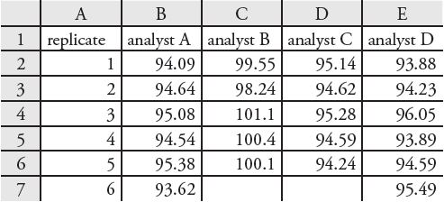
Figure 14.22 Portion of a spreadsheet containing the data from Table 14.6.

Figure 14.23 Output from Excel’s one-way analysis of variance of the data in Table 14.6. The summary table provides the mean and variance for each analyst. The ANOVA table summarizes the sum-of-squares terms (SS), the degrees of freedom (df), the variances (MS for mean square), the value of Fexp and the critical value of F, and the probability of incorrectly rejecting the null hypothesis that there is no significant difference between the analysts.
14.4.2 R
To complete an analysis of variance for the data in Table 14.6 using R, we first need to create several objects. The first object contains each result from Table 14.6.
> results=c(94.090, 94.640, 95.008, 94.540, 95.380, 93.620, 99.550, 98.240, 101.100, 100.400, 100.100, 95.140, 94.620, 95.280, 94.590, 94.240, 93.880, 94.230, 96.050, 93.890, 94.950, 95.490)
Note
You can arrange the results in any order. In creating this object, I choose to list the results for analyst A, followed by the results for analyst B, C, and D.
The second object contains labels to identify the source of each entry in the first object. The following code creates this object.
> analyst = c(rep(“a”,6), rep(“b”,5), rep(“c”,5), rep(“d”,6))
Note
The command rep (for repeat) has two variables: the item to repeat and the number of times it is repeated. The object analyst is the vector (“a”,“a”,“a”,“a”,“a”,“a”, “b”,“b”,“b”,“b”,“b”, “c”, “c”,“c”,“c”,“c”,“d”, “d”, “d”, “d”, “d”, “d”).
Next, we combine the two objects into a table with two columns, one containing the data (results) and one containing the labels (analyst).
> df = data.frame(results, labels = factor(analyst))
Note
We call this table a data frame. Many functions in R work on the columns in a data frame.
The command factor indicates that the object analyst contains the categorical factors for the analysis of variance. The command for an analysis of variance takes the following form
anova(lm(data ~ factors), data = data.frame)
where data and factors are the columns containing the data and the categorical factors, and data.frame is the name we assigned to the data table. Figure 14.24 shows the output for an analysis of variance of the data in Table 14.6. The small value of 3.04×10⁻⁹ for falsely rejecting the null hypothesis indicates that there is a significant source of variation between the analysts.
Note
The command lm stands for linear model. See Section 5.6.2 in Chapter 5 for a discussion of linear models in R.
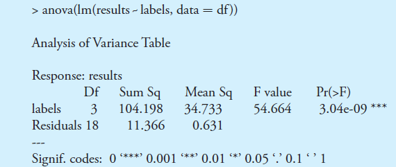
Figure 14.24 Output of an R session for an analysis of variance for the data in Table 14.6. In the table, “labels” is the between-sample variance and “residuals” is the within-sample variance. The p-value of 3.04e-09 is the probability of incorrectly rejecting the null hypothesis that the within-sample and between-sample variances are the same.
Having found a significant difference between the analysts, we want to identify the source of this difference. R does not include Fisher’s least significant difference test, but it does include a function for a related method called Tukey’s honest significant difference test. The command for this test takes the following form
> TukeyHSD(aov(lm(data ~ factors), data = data.frame), conf.level = 0.95)
where data and factors are the columns containing the data and the categorical factors, and data.frame is the name we assigned to the data table.
Note
You may recall that an underlined command is the default value. If you are using an α of 0.05 (a 95% confidence level), then you do not need to include the entry for conf.level. If you wish to use an α of 0.10, then enter conf.level = 0.90.
Figure 14.25 shows the output of this command and its interpretation. The small probability values when comparing analyst B to each of the other analysts indicates that this is the source of the significant difference identified in the analysis of variance.
Note
Note that p value is small when the confidence interval for the difference includes zero.
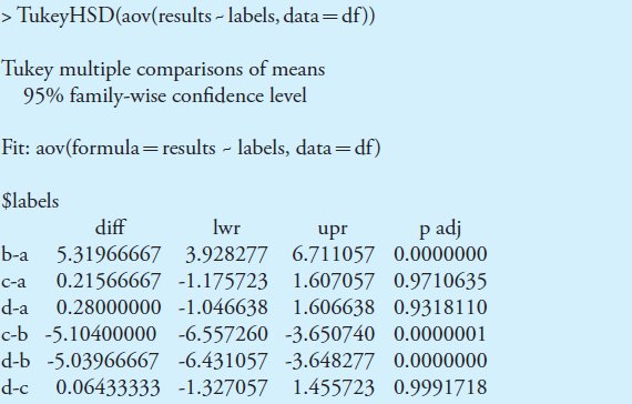
Figure 14.25 Output of an R session for a Tukey honest significance difference test for the data in Table 14.6. For each possible comparison of analysts, the table gives the actual difference between the analysts, “diff,” and the smallest, “lwr,” and the largest, “upr,” differences for a 95% confidence interval. The “p adj” is the probability that a difference of zero falls within this confidence interval. The smaller the p-value, the greater the probability that the difference between the analysts is significant.