EPR - Interpretation

Introduction

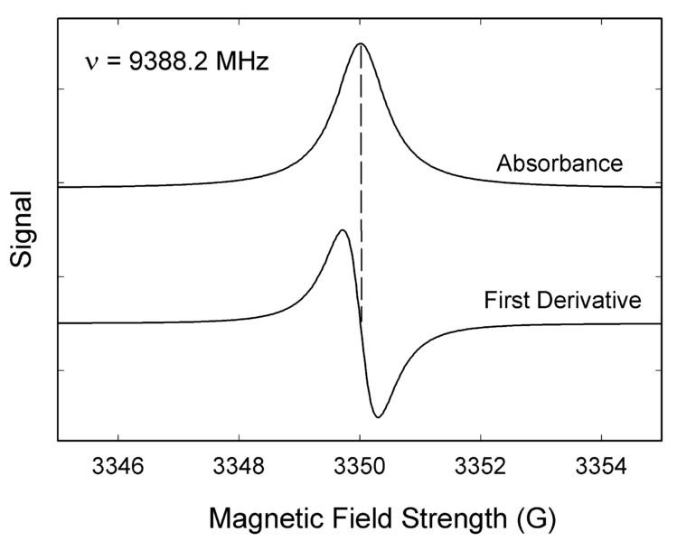
Like most spectroscopic techniques, EPR spectrometers measure the absorption of electromagnetic radiation. A simple absorption spectra will appear similar to the one on the top of Figure 1. However, a phase-sensitive detector is used in EPR spectrometers which converts the normal absorption signal to its first derivative. Then the absorption signal is presented as its first derivative in the spectrum, which is similar to the one on the bottom of Figure 1. Thus, the magnetic field is on the x-axis of EPR spectrum; dχ″/dB, the derivative of the imaginary part of the molecular magnetic susceptibility with respect to the external static magnetic field in arbitrary units is on the y-axis. In the EPR spectrum, where the spectrum passes through zero corresponds to the absorption peak of absorption spectrum. People can use this to determine the center of the signal. On the x-axis, sometimes people use the unit “gauss” (G), instead of tesla (T). One tesla is equal to 10000 gauss.

Proportionality factor (g-factor)

As a result of the Zeeman Effect, the state energy difference of an electron with s=1/2 in magnetic field is

\[ \Delta E = gβB \label{1}\]

where β is the constant, Bohr magneton. Since the energy absorbed by the electron should be exactly the same with the state energy difference ΔE, ΔE=hv ( h is Planck’s constant), the Equation \(\ref{1}\) can be expressed as

\[ h \nu=gβB \label{2} \]

People can control the microwave frequency v and the magnetic field \(B\). The other factor, \(g\), is a constant of proportionality, whose value is the property of the electron in a certain environment. After plugging in the values of \(h\) and \(β\) in Equation \(\ref{2}\), g value can be given through Equation \(\ref{3}\):

\[ g = 71.4484v \text{(in GHz)/B (in mT)} \label{3} \]

A free electron in vacuum has a \(g\) value (\(g_e= 2.00232\). For instance, at the magnetic field of 331.85 mT, a free electron absorbs the microwave with an X-band frequency of 9.300 GHz. However, when the electron is in a certain environment, for example, a transition metal-ion complex, the second magnetic field produced by the nuclei, ΔB, will also influence the electron. At this kind of circumstance, Equation \(\ref{2}\) becomes

\[ h\nu = gβ(B_e+ \Delta B) \label{4} \]

since we only know the spectrometer value of B, the Equation \(\ref{4}\) is written as:

\[ h\nu = (g_e+ \Delta g)βB ] \label{5}\]

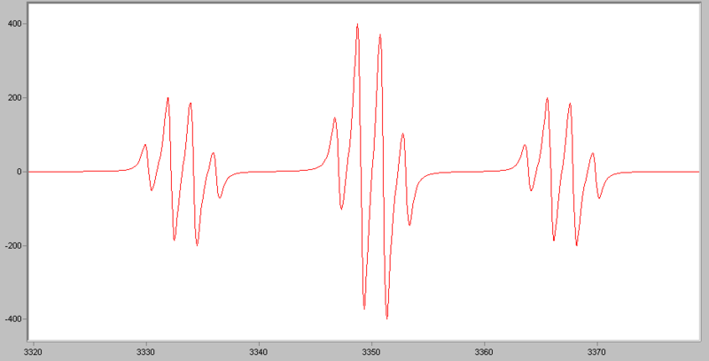
From the relationship shown above, we know that there are infinite pairs of v and B that fit this relationship. The magnetic field for resonance is not a unique “fingerprint” for the identification of a compound because spectra can be acquired at different microwave frequencies. Then what is the fingerprint of a molecule? It is Δg. This value contains the chemical information that lies in the interaction between the electron and the electronic structure of the molecule, one can simply take the value of g = g_e+ Δg as a fingerprint of the molecule. For organic radicals, the g value is very close to ge with values ranging from 1.99-2.01. For example, the g value for •CH3 is 2.0026. For transition metal complexes, the g value varies a lot because of the spin-orbit coupling and zero-field splitting. Usually it ranges from 1.4-3.0, depending on the geometry of the complex. For instance, the g value of Cu(acac)2 is 2.13. To determine the g value, we use the center of the signal. By using Equation \(\ref{3}\), we can calculate the g factor of the absorption in the spectrum. The value of g factor is not only related to the electronic environment, but also related to anisotropy. About this part, please refer to EPR:Theory, Parallel Mode EPR: Theory and ENDOR:Theory. An example from UC Davis is shown below[1] (Britt group, Published in J.A.C.S. ):

Hyperfine Interactions

Another very important factor in EPR is hyperfine interactions. Besides the applied magnetic field B₀, the compound contains the unpaired electrons are sensitive to their local “micro” environment. Additional information can be obtained from the so-called hyperfine interaction. The nuclei of the atoms in a molecule or complex usually have their own fine magnetic moments. Such magnetic moments occurrence can produce a local magnetic field intense enough to affect the electron. Such interaction between the electron and the nuclei produced local magnetic field is called the hyperfine interaction. Then the energy level of the electron can be expressed as:

\[E = gm_BB_0M_S + aM_sm_I \label{6}\]

with \(a\) is the hyperfine coupling constant, \(m_I\) is the nuclear spin quantum number.

Hyperfine interactions can be used to provide a wealth of information about the sample such as the number and identity of atoms in a molecule or compound, as well as their distance from the unpaired electron.

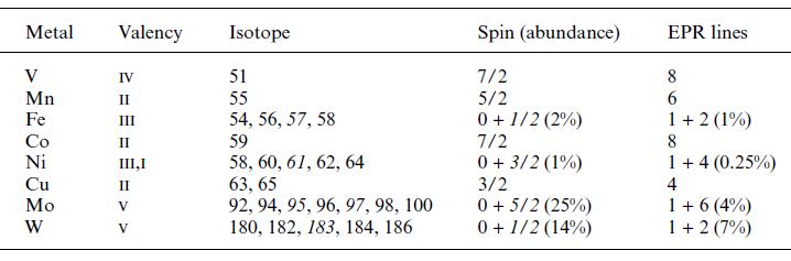
Table 1. Bio transition metal nuclear spins and EPR hyperfine patterns^[3]

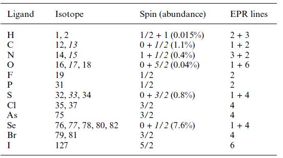
The rules for determining which nuclei will interact are the same as for NMR. For isotopes which have even atomic and even mass numbers, the ground state nuclear spin quantum number, I, is zero, and these isotopes have no EPR (or NMR) spectra. For isotopes with odd atomic numbers and even mass numbers, the values of I are integers. For example the spin of ²H is 1. For isotopes with odd mass numbers, the values of I are fractions. For example the spin of ¹H is 1/2 and the spin of ²³Na is 7/2. Here are more examples from biological systems:

Table 2. Bio ligand atom nuclear spins and their EPR hyperfine patterns^[3]

The number of lines from the hyperfine interaction can be determined by the formula: 2NI + 1. N is the number of equivalent nuclei and I is the spin. For example, an unpaired electron on a V⁴⁺ experiences I=7/2 from the vanadium nucleus. We can see 8 lines from the EPR spectrum. When coupling to a single nucleus, each line has the same intensity. When coupling to more than one nucleus, the relative intensity of each line is determined by the number of interacting nuclei. For the most common I=1/2 nuclei, the intensity of each line follows Pascal's triangle, which is shown below:

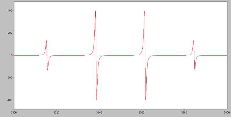
For example, for •CH₃, the radical’s signal is split to 2NI+1= 2*3*1/2+1=4 lines, the ratio of each line’s intensity is 1:3:3:1. The spectrum looks like this:

If an electron couples to several sets of nuclei, first we apply the coupling rule to the nearest nuclei, then we split each of those lines by the coupling them to the next nearest nuclei, and so on. For the methoxymethyl radical, H₂C(OCH₃), there are (2*2*1/2+1)*(2*3*1/2+1)=12 lines in the spectrum, the spectrum looks like this:

For I=1, the relative intensities follow this triangle:

The EPR spectra have very different line shapes and characteristics depending on many factors, such as the interactions in the spin Hamiltonian, physical phase of samples, dynamic properties of molecules. To gain the information on structure and dynamics from experimental data, spectral simulations are heavily relied. People use simulation to study the dependencies of spectral features on the magnetic parameters, to predict the information we may get from experiments, or to extract accurate parameter from experimental spectra.

References

1. Dicus, M.M; Conlan,A.; Nechushtai,R.; Jennings,P.A.;Paddock,M.L.; Britt,R.D.; Stoll S. J. AM. CHEM. SOC. 2010, 132, 2037–2049
2. Hagen,W.R. 2009. Biomolecular EPR Spectroscopy. Boca Raton: CRC Press.
3. Hagen,W.R. Dalton Trans., 2006, 4415–4434
4. Stoll,S., Schweiger,A. Journal of Magnetic Resonance 178 (2006) 42–55