3.2.6: Steady State Approximation

Last updated
Save as PDF

Page ID: 1420

\( \newcommand{\vecs}[1]{\overset { \scriptstyle \rightharpoonup} {\mathbf{#1}} } \) \( \newcommand{\vecd}[1]{\overset{-\!-\!\rightharpoonup}{\vphantom{a}\smash {#1}}} \)\(\newcommand{\id}{\mathrm{id}}\) \( \newcommand{\Span}{\mathrm{span}}\) \( \newcommand{\kernel}{\mathrm{null}\,}\) \( \newcommand{\range}{\mathrm{range}\,}\) \( \newcommand{\RealPart}{\mathrm{Re}}\) \( \newcommand{\ImaginaryPart}{\mathrm{Im}}\) \( \newcommand{\Argument}{\mathrm{Arg}}\) \( \newcommand{\norm}[1]{\| #1 \|}\) \( \newcommand{\inner}[2]{\langle #1, #2 \rangle}\) \( \newcommand{\Span}{\mathrm{span}}\) \(\newcommand{\id}{\mathrm{id}}\) \( \newcommand{\Span}{\mathrm{span}}\) \( \newcommand{\kernel}{\mathrm{null}\,}\) \( \newcommand{\range}{\mathrm{range}\,}\) \( \newcommand{\RealPart}{\mathrm{Re}}\) \( \newcommand{\ImaginaryPart}{\mathrm{Im}}\) \( \newcommand{\Argument}{\mathrm{Arg}}\) \( \newcommand{\norm}[1]{\| #1 \|}\) \( \newcommand{\inner}[2]{\langle #1, #2 \rangle}\) \( \newcommand{\Span}{\mathrm{span}}\)\(\newcommand{\AA}{\unicode[.8,0]{x212B}}\)

The steady state approximation is a method used to estimate the overall reaction rate of a multi-step reaction. It assumes that the rate of change of intermediate concentration in a multi-step reaction are constant. This method can only be applied when the first step of the reaction is significantly slower than subsequent step in an intermediate-forming consecutive reaction.

Introduction

Before discussing the steady state approximation, it must be understood that the approximation is derived to simplify the kinetic expression for product concentration, [product]. Consider the following sequential reaction:

\[A \xrightarrow[]{k_1} B \xrightarrow {k_2} C \nonumber \]

Calculating the [product] depends on all the rate constants in each step. For example, if the kinetic method was used to find the concentration of C, [C], at time t in the above reaction, the expression would be

\[[C] = [A]_0 \left(1+ \dfrac{k_2e^{-k_1t}-k_1e^{-k_2t})}{k_1 - k_2}\right) \label{1} \]

With a more complicated mechanisms, the kinetic expression becomes harder to derive. To simplify this calculation, we often use one of two approximations for determining the overall reaction rates of consecutive reactions: the steady state approximation and the pre-equilibrium approximation. This article concerns the steady state approximation.

Steady State Approximation

The steady state approximation is applies to a consecutive reaction with a slow first step and a fast second step (\(k_1 \ll k_2\)). If the first step is very slow in comparison to the second step, there is no accumulation of intermediate product, such as product B in the above example.

\[\dfrac{d[B]}{dt} = 0 = k_1[A] - k_2[B] \label{2} \]

Thus

\[[B] = \dfrac{k_1[A]}{k_2} \label{3} \]

From the mechanism:

\[\dfrac{d[C]}{dt} = k_2[B] = \dfrac{k_2k_1[A]}{k_2} = k_1[A] \label{4} \]

Solving for \([C]\):

\[[C] = [A]_0 (1- e^{-k_1t}) \label{5} \]

Equation \(\ref{5}\) is much simpler to derive than Equation \(\ref{1}\), especially with a more complicated multi-step reaction mechanisms.

Example \(\PageIndex{1}\)

Consider the reaction:

\[A + 2B \xrightarrow[]{} C \nonumber \]

What is the expected rate law according to the following proposed multi-step mechanism under the steady state approximation with \(k_2 \gg k_{-1}\)) for the following mechanism: \[A + B \ce{<=>[k_1][k_{-1}]} I \tag{Slow} \] \[I + B \xrightarrow[]{k_2} C \tag{Fast} \]
If \(x\) is the order of the reaction with respect to \(A\), \(y\) is the order of the reaction with respect to \(B\), and \(n\) is the overall reaction order. What are the values of \(x\), \(y\), and \(n\)?

Solution

a: First we use the Steady State Approximation for the intermediate (i.e., Equation \ref{2})

\[\dfrac{d[I]}{dt} = k_1[A][B] - k_{-1}[I] - k_2[I][B] = 0 \nonumber \]

then we solve for the (steady-state) concentration of the intermediate

\[[I] = \dfrac{k_1[A][B]}{ k_{-1} +k_2[B]} \nonumber \]

Because the second step is much faster than the first step, then \(k_2 \gg k_{-1}\) then \(k_{-1} \approx 0\) for this approximation and the above equation can be simplified to

\[[I] = \dfrac{k_1[A]}{k_2} \nonumber. \nonumber \]

The rate law for the production of \([C]\) can be constructed directly from the second step and when the steady-state concentration of \(I\) is added, the final rate law expression is derived.

\[ \begin{align*}\dfrac{d[C]}{dt} & = k_2[I][B] \\[4pt] &= \dfrac{k_1k_2[A][B]}{k_2} \\[4pt] &= k_1[A][B] \end{align*} \]

b: Direct inspection of the final rate law derived above gives these parameters:

\(x = 1\)
\(y = 1\)
\(n = 2\)

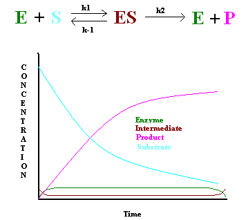
Use of the Steady-State Approximation in Enzyme Kinetics

In 1925, George E. Briggs and John B. S. Haldane applied the steady state approximation method to determine the rate law of the enzyme-catalyzed reaction (Figure 1). The following assumptions were made:

The rate constant of the first step must be slower than the rate constant of the second step (\(k_1 \ll k_2\)), hence \[\dfrac{d[ES]}{dt} = 0 \nonumber \]
Enzyme concentration must be significantly lower than the substrate concentration to keep the first step slower than the second step.

Figure 1: Steady state dynamics in enzymes

This gives the following:

\[\dfrac{d[P]}{dt} = k_2[ES] \label{6} \]

where

\[\dfrac{d[ES]}{dt} = 0 = k_1[E][S] - k_{-1}[ES] - k_2[ES] \label{7} \]

Because

\[[S] \gg [E] \label{8} \]

Using the second assumption and the fact that enzyme concentration equals the initial concentration of enzyme minus the concentration of the enzyme-substrate intermediate,

\[[E] = [E]_o - [ES] \label{9} \]

The following equation is obtained:

\[k_1[E]_o[S] = k_{-1}[ES] + k_2[ES] + k_1[ES][S] \label{10} \]

From this equation, the concentration of the ES intermediate can be found:

\[[ES] = \dfrac{k_1[E]_o[S]}{(k_{-1} + k_2) + k_1[S]} \label{11} \]

Substitute this into Equation \(\ref{6}\) gives,

\[\dfrac{d[P]}{dt} = \dfrac{k_2[E]_0[S]}{[(k_1+k_2)/k_1]+[S]} = \dfrac{k_2[E]_0[S]}{K_M+[S]} \label{12} \]

where

\[K_M = \dfrac{k_{-1}+k_{2}}{k_1} \label{13} \]

Because in most of the cases, only the initial \(d[P]/dt\) is measured to determine the rate of product formation, Equation \ref{12} can be rewritten as:

\[v_o = \dfrac{d[P]_0}{dt} = \dfrac{k_2[E]_0[S]}{K_M+[S]} \label{14} \]

Because \([E]_o = v_{max}/k_2\). Equation \(\ref{14}\) becomes the following:

\[ \begin{align} v_0 &= \dfrac{d[P]_o}{dt} \\[4pt] &= \dfrac{(k_2/k_2)v_{max}[S]}{K_M+[S]} \label{15} \\ &= \dfrac{v_{max}[S]}{K_M+[S]} \label{16} \end{align} \]

This equation is a useful tool to in calculating \(v_{max}\) and \(K_M\) (the Michaelis constant) of an enzyme by using the Lineweaver-Burk plot (1/[S] vs. 1/v₀) or the Eadie-Hofstee plot (v₀/[S] vs. v₀).

Problems

Given the reaction \(A \xrightarrow[]{k_1} B \xrightarrow[]{k_2} C\)

where k₁= 0.2 M^-1s^-1 , k₂ = 2000 s^-1

Write the reaction rates for A, B, and C.
Is this a steady-state reaction?
Write the expression for d[C]/dt using the Steady State Approximation
Calculate d[C]/dt if [A] = 1M
Calculate [C] at t = 3 s and [A]₀ = 2M

Solutions

1) d[A]/dt = -k₁[A]; d[B]/dt = k₁[A] - k₂[B]; d[C]/dt = k₂[B]

2) Because k₁ is much larger than k₂, this is a steady state reaction.

3) d[C]/dt = k₂[B]

where d[B]/dt = k₁[A] - k₂[B] = 0

so, [B] = k₁[A]/k₂

Substitute this into d[C]/dt

d[C]/dt = k₁[A]

4) d[C]/dt = 0.2M^-1s^-1(1M) = 0.2 s^-1

5) [C] = [A]₀ (1-e^-k₁t) = 2M(1-e^-0.2(3)) = 0.9 M

References:

Chang, Raymond. Physical Chemistry for The Biosciences. Sausalito: University Science Books, 2005. 368-370.
Garrett, Reginald H, Charles M. Grisham. Biochemistry. 4^{th ed.} Boston: Brooks/Cole Cengage Learning, 2010. 389-397.
Segel, Irwin H. Biochemical Calculations. 2^nd ed. New Jersey: John Wiley and Sons, inc., 1976. 216-218.