
14.5: Temperature and Rate
- Page ID
- 25179
- To understand why and how chemical reactions occur.
It is possible to use kinetics studies of a chemical system, such as the effect of changes in reactant concentrations, to deduce events that occur on a microscopic scale, such as collisions between individual particles. Such studies have led to the collision model of chemical kinetics, which is a useful tool for understanding the behavior of reacting chemical species. The collision model explains why chemical reactions often occur more rapidly at higher temperatures. For example, the reaction rates of many reactions that occur at room temperature approximately double with a temperature increase of only 10°C. In this section, we will use the collision model to analyze this relationship between temperature and reaction rates. Before delving into the relationship between temperature and reaction rate, we must discuss three microscopic factors that influence the observed macroscopic reaction rates.
Microscopic Factor 1: Collisional Frequency
Central to collision model is that a chemical reaction can occur only when the reactant molecules, atoms, or ions collide. Hence, the observed rate is influence by the frequency of collisions between the reactants. The collisional frequency is the average rate in which two reactants collide for a given system and is used to express the average number of collisions per unit of time in a defined system. While deriving the collisional frequency (\(Z_{AB}\)) between two species in a gas is straightforward, it is beyond the scope of this text and the equation for collisional frequency of \(A\) and \(B\) is the following:
\[Z_{AB} = N_{A}N_{B}\left(r_{A} + r_{B}\right)^2\sqrt{ \dfrac{8\pi k_{B}T}{\mu_{AB}}} \label{freq} \]
with
- \(N_A\) and \(N_B\) are the numbers of \(A\) and \(B\) molecules in the system, respectively
- \(r_a\) and \(r_b\) are the radii of molecule \(A\) and \(B\), respectively
- \(k_B\) is the Boltzmann constant \(k_B\) =1.380 x 10⁻²³ Joules Kelvin
- \(T\) is the temperature in Kelvin
- \(\mu_{AB}\) is calculated via \(\mu_{AB} = \frac{m_Am_B}{m_A + m_B}\)
The specifics of Equation \ref{freq} are not important for this conversation, but it is important to identify that \(Z_{AB}\) increases with increasing density (i.e., increasing \(N_A\) and \(N_B\)), with increasing reactant size (\(r_a\) and \(r_b\)), with increasing velocities (predicted via Kinetic Molecular Theory), and with increasing temperature (although weakly because of the square root function).
A Video Discussing Collision Theory of Kinetics: Collusion Theory of Kinetics (opens in new window) [youtu.be]
Microscopic Factor 2: Activation Energy
Previously, we discussed the kinetic molecular theory of gases, which showed that the average kinetic energy of the particles of a gas increases with increasing temperature. Because the speed of a particle is proportional to the square root of its kinetic energy, increasing the temperature will also increase the number of collisions between molecules per unit time. What the kinetic molecular theory of gases does not explain is why the reaction rate of most reactions approximately doubles with a 10°C temperature increase. This result is surprisingly large considering that a 10°C increase in the temperature of a gas from 300 K to 310 K increases the kinetic energy of the particles by only about 4%, leading to an increase in molecular speed of only about 2% and a correspondingly small increase in the number of bimolecular collisions per unit time.
The collision model of chemical kinetics explains this behavior by introducing the concept of activation energy (\(E_a\)). We will define this concept using the reaction of \(\ce{NO}\) with ozone, which plays an important role in the depletion of ozone in the ozone layer:
\[\ce{NO(g) + O_3(g) \rightarrow NO_2(g) + O_2(g)} \nonumber \]
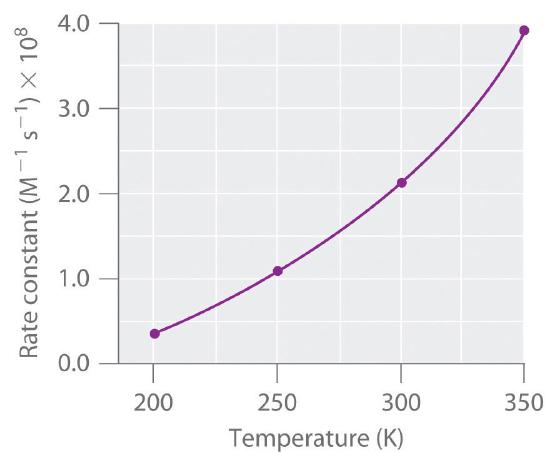
Increasing the temperature from 200 K to 350 K causes the rate constant for this particular reaction to increase by a factor of more than 10, whereas the increase in the frequency of bimolecular collisions over this temperature range is only 30%. Thus something other than an increase in the collision rate must be affecting the reaction rate.
Experimental rate law for this reaction is
\[\text{rate} = k [\ce{NO}][\ce{O3}] \nonumber \]
and is used to identify how the reaction rate (not the rate constant) vares with concentration. The rate constant, however, does vary with temperature. Figure \(\PageIndex{1}\) shows a plot of the rate constant of the reaction of \(\ce{NO}\) with \(\ce{O3}\) at various temperatures. The relationship is not linear but instead resembles the relationships seen in graphs of vapor pressure versus temperature (e.g, the Clausius-Claperyon equation). In all three cases, the shape of the plots results from a distribution of kinetic energy over a population of particles (electrons in the case of conductivity; molecules in the case of vapor pressure; and molecules, atoms, or ions in the case of reaction rates). Only a fraction of the particles have sufficient energy to overcome an energy barrier.
In the case of vapor pressure, particles must overcome an energy barrier to escape from the liquid phase to the gas phase. This barrier corresponds to the energy of the intermolecular forces that hold the molecules together in the liquid. In conductivity, the barrier is the energy gap between the filled and empty bands. In chemical reactions, the energy barrier corresponds to the amount of energy the particles must have to react when they collide. This energy threshold, called the activation energy, was first postulated in 1888 by the Swedish chemist Svante Arrhenius (1859–1927; Nobel Prize in Chemistry 1903). It is the minimum amount of energy needed for a reaction to occur. Reacting molecules must have enough energy to overcome electrostatic repulsion, and a minimum amount of energy is required to break chemical bonds so that new ones may be formed. Molecules that collide with less than the threshold energy bounce off one another chemically unchanged, with only their direction of travel and their speed altered by the collision. Molecules that are able to overcome the energy barrier are able to react and form an arrangement of atoms called the activated complex or the transition state of the reaction. The activated complex is not a reaction intermediate; it does not last long enough to be detected readily.
Any phenomenon that depends on the distribution of thermal energy in a population of particles has a nonlinear temperature dependence.
We can graph the energy of a reaction by plotting the potential energy of the system as the reaction progresses. Figure \(\PageIndex{2}\) shows a plot for the NO–O3 system, in which the vertical axis is potential energy and the horizontal axis is the reaction coordinate, which indicates the progress of the reaction with time. The activated complex is shown in brackets with an asterisk. The overall change in potential energy for the reaction (\(ΔE\)) is negative, which means that the reaction releases energy. (In this case, \(ΔE\) is −200.8 kJ/mol.) To react, however, the molecules must overcome the energy barrier to reaction (\(E_a\) is 9.6 kJ/mol). That is, 9.6 kJ/mol must be put into the system as the activation energy. Below this threshold, the particles do not have enough energy for the reaction to occur.
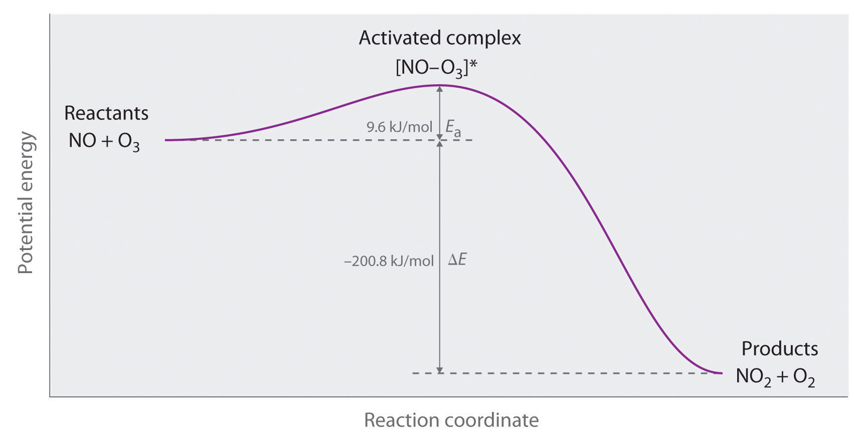
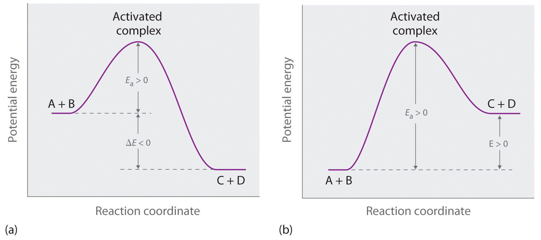
Figure \(\PageIndex{3a}\) illustrates the general situation in which the products have a lower potential energy than the reactants. In contrast, Figure \(\PageIndex{3b}\) illustrates the case in which the products have a higher potential energy than the reactants, so the overall reaction requires an input of energy; that is, it is energetically uphill, and \(ΔE > 0\). Although the energy changes that result from a reaction can be positive, negative, or even zero, in most cases an energy barrier must be overcome before a reaction can occur. This means that the activation energy is almost always positive; there is a class of reactions called barrierless reactions, but those are discussed elsewhere.
For similar reactions under comparable conditions, the one with the smallest Ea will occur most rapidly.
Whereas \(ΔE\) is related to the tendency of a reaction to occur spontaneously, \(E_a\) gives us information about the reaction rate and how rapidly the reaction rate changes with temperature. For two similar reactions under comparable conditions, the reaction with the smallest \(E_a\) will occur more rapidly.
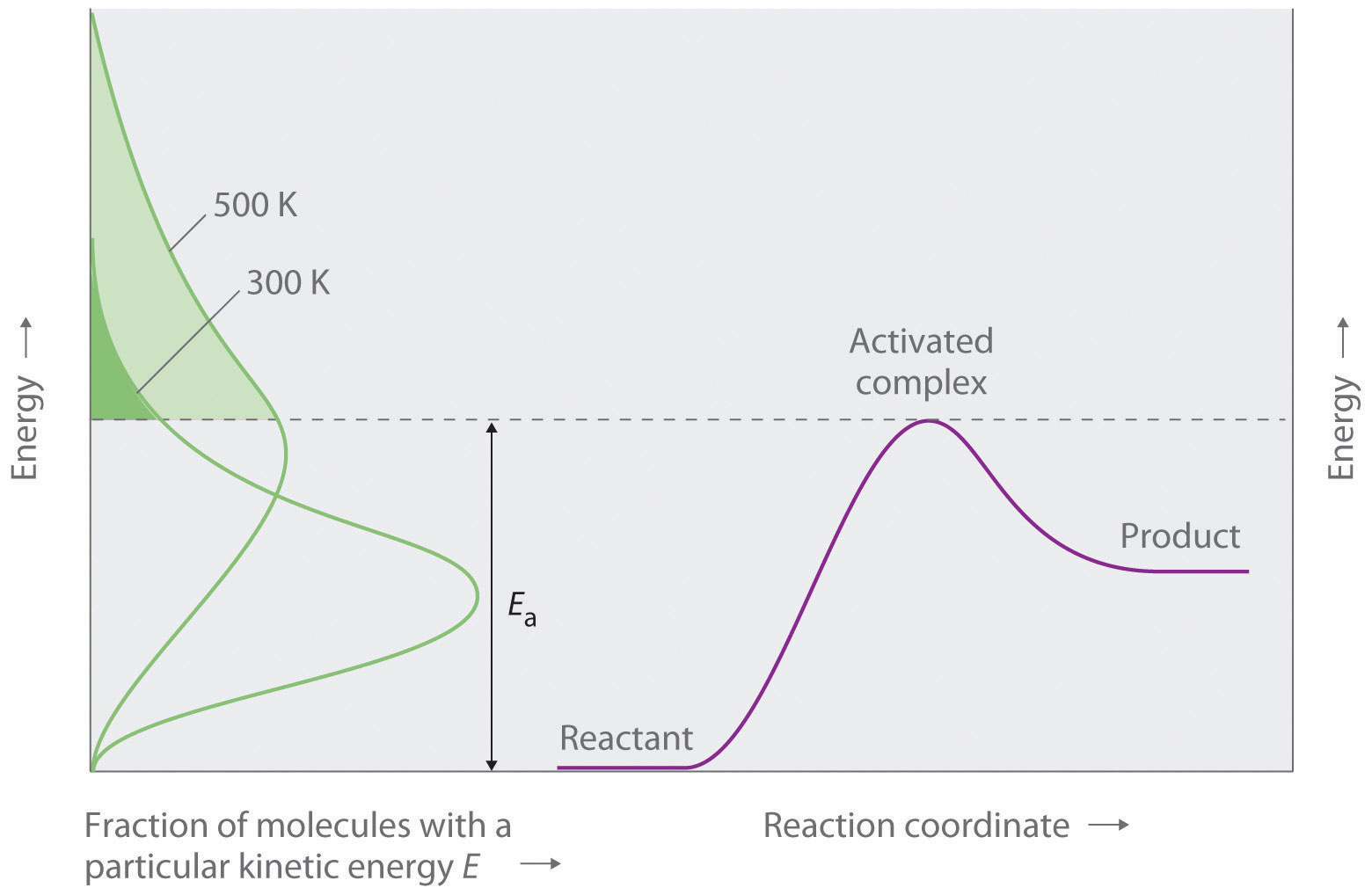
Figure \(\PageIndex{4}\) shows both the kinetic energy distributions and a potential energy diagram for a reaction. The shaded areas show that at the lower temperature (300 K), only a small fraction of molecules collide with kinetic energy greater than Ea; however, at the higher temperature (500 K) a much larger fraction of molecules collide with kinetic energy greater than Ea. Consequently, the reaction rate is much slower at the lower temperature because only a relatively few molecules collide with enough energy to overcome the potential energy barrier.
Video Discussing Transition State Theory: Transition State Theory(opens in new window) [youtu.be]
Microscopic Factor 3: Sterics
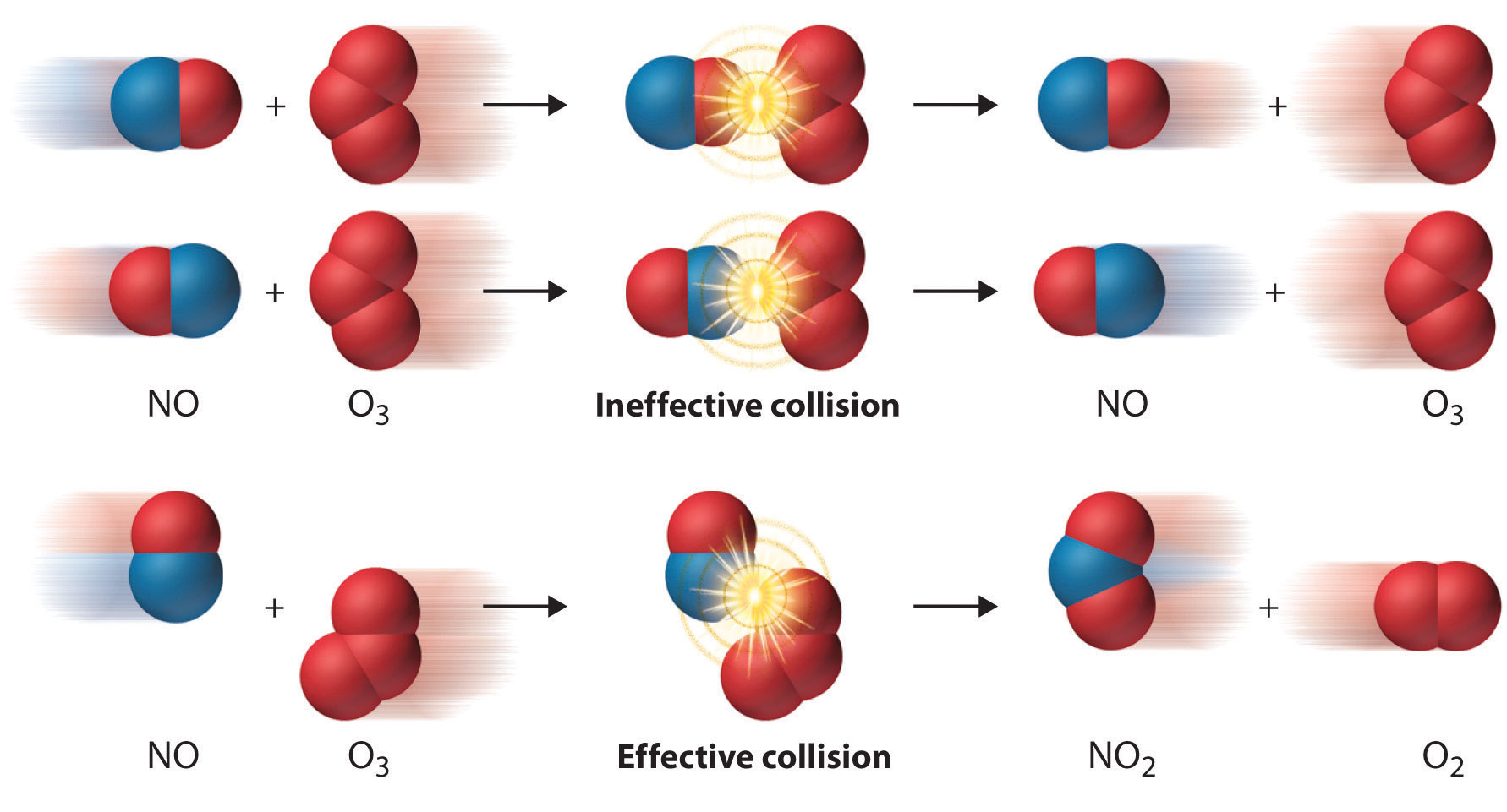
Even when the energy of collisions between two reactant species is greater than \(E_a\), most collisions do not produce a reaction. The probability of a reaction occurring depends not only on the collision energy but also on the spatial orientation of the molecules when they collide. For \(\ce{NO}\) and \(\ce{O3}\) to produce \(\ce{NO2}\) and \(\ce{O2}\), a terminal oxygen atom of \(\ce{O3}\) must collide with the nitrogen atom of \(\ce{NO}\) at an angle that allows \(\ce{O3}\) to transfer an oxygen atom to \(\ce{NO}\) to produce \(\ce{NO2}\) (Figure \(\PageIndex{4}\)). All other collisions produce no reaction. Because fewer than 1% of all possible orientations of \(\ce{NO}\) and \(\ce{O3}\) result in a reaction at kinetic energies greater than \(E_a\), most collisions of \(\ce{NO}\) and \(\ce{O3}\) are unproductive. The fraction of orientations that result in a reaction is called the steric factor (\(\rho\)) and its value can range from \(\rho=0\) (no orientations of molecules result in reaction) to \(\rho=1\) (all orientations result in reaction).
Macroscopic Behavior: The Arrhenius Equation
The collision model explains why most collisions between molecules do not result in a chemical reaction. For example, nitrogen and oxygen molecules in a single liter of air at room temperature and 1 atm of pressure collide about 1030 times per second. If every collision produced two molecules of \(\ce{NO}\), the atmosphere would have been converted to \(\ce{NO}\) and then \(\ce{NO2}\) a long time ago. Instead, in most collisions, the molecules simply bounce off one another without reacting, much as marbles bounce off each other when they collide.
For an \(A + B\) elementary reaction, all three microscopic factors discussed above that affect the reaction rate can be summarized in a single relationship:
\[\text{rate} = (\text{collision frequency}) \times (\text{steric factor}) \times (\text{fraction of collisions with } E > E_a ) \nonumber \]
where
\[\text{rate} = k[A][B] \label{14.5.2} \]
Arrhenius used these relationships to arrive at an equation that relates the magnitude of the rate constant for a reaction to the temperature, the activation energy, and the constant, \(A\), called the frequency factor:
\[k=Ae^{-E_{\Large a}/RT} \label{14.5.3} \]
The frequency factor is used to convert concentrations to collisions per second (scaled by the steric factor). Because the frequency of collisions depends on the temperature, \(A\) is actually not constant (Equation \ref{freq}). Instead, \(A\) increases slightly with temperature as the increased kinetic energy of molecules at higher temperatures causes them to move slightly faster and thus undergo more collisions per unit time.
Equation \(\ref{14.5.3}\) is known as the Arrhenius equation and summarizes the collision model of chemical kinetics, where \(T\) is the absolute temperature (in K) and R is the ideal gas constant [8.314 J/(K·mol)]. \(E_a\) indicates the sensitivity of the reaction to changes in temperature. The reaction rate with a large \(E_a\) increases rapidly with increasing temperature, whereas the reaction rate with a smaller \(E_a\) increases much more slowly with increasing temperature.
If we know the reaction rate at various temperatures, we can use the Arrhenius equation to calculate the activation energy. Taking the natural logarithm of both sides of Equation \(\ref{14.5.3}\),
\[\begin{align} \ln k &=\ln A+\left(-\dfrac{E_{\textrm a}}{RT}\right) \\[4pt] &=\ln A+\left[\left(-\dfrac{E_{\textrm a}}{R}\right)\left(\dfrac{1}{T}\right)\right] \label{14.5.4} \end{align} \]
Equation \(\ref{14.5.4}\) is the equation of a straight line,
\[y = mx + b \nonumber \]
where \(y = \ln k\) and \(x = 1/T\). This means that a plot of \(\ln k\) versus \(1/T\) is a straight line with a slope of \(−E_a/R\) and an intercept of \(\ln A\). In fact, we need to measure the reaction rate at only two temperatures to estimate \(E_a\).
Knowing the \(E_a\) at one temperature allows us to predict the reaction rate at other temperatures. This is important in cooking and food preservation, for example, as well as in controlling industrial reactions to prevent potential disasters. The procedure for determining \(E_a\) from reaction rates measured at several temperatures is illustrated in Example \(\PageIndex{1}\).
A Video Discussing The Arrhenius Equation: The Arrhenius Equation(opens in new window) [youtu.be]
Many people believe that the rate of a tree cricket’s chirping is related to temperature. To see whether this is true, biologists have carried out accurate measurements of the rate of tree cricket chirping (\(f\)) as a function of temperature (\(T\)). Use the data in the following table, along with the graph of ln[chirping rate] versus \(1/T\) to calculate \(E_a\) for the biochemical reaction that controls cricket chirping. Then predict the chirping rate on a very hot evening, when the temperature is 308 K (35°C, or 95°F).
| Frequency (f; chirps/min) | ln f | T (K) | 1/T (K) |
|---|---|---|---|
| 200 | 5.30 | 299 | 3.34 × 10⁻³ |
| 179 | 5.19 | 298 | 3.36 × 10⁻³ |
| 158 | 5.06 | 296 | 3.38 × 10⁻³ |
| 141 | 4.95 | 294 | 3.40 × 10⁻³ |
| 126 | 4.84 | 293 | 3.41 × 10⁻³ |
| 112 | 4.72 | 292 | 3.42 × 10⁻³ |
| 100 | 4.61 | 290 | 3.45 × 10⁻³ |
| 89 | 4.49 | 289 | 3.46 × 10⁻³ |
| 79 | 4.37 | 287 | 3.48 × 10⁻³ |
Given: chirping rate at various temperatures
Asked for: activation energy and chirping rate at specified temperature
Strategy:
- From the plot of \(\ln f\) versus \(1/T\), calculate the slope of the line (−Ea/R) and then solve for the activation energy.
- Express Equation \ref{14.5.4} in terms of k1 and T1 and then in terms of k2 and T2.
- Subtract the two equations; rearrange the result to describe k2/k1 in terms of T2 and T1.
- Using measured data from the table, solve the equation to obtain the ratio k2/k1. Using the value listed in the table for k1, solve for k2.
Solution
A If cricket chirping is controlled by a reaction that obeys the Arrhenius equation, then a plot of \(\ln f\) versus \(1/T\) should give a straight line (Figure \(\PageIndex{6}\)).

Also, the slope of the plot of \(\ln f\) versus \(1/T\) should be equal to \(−E_a/R\). We can use the two endpoints in Figure \(\PageIndex{6}\) to estimate the slope:
\[\begin{align*}\textrm{slope}&=\dfrac{\Delta\ln f}{\Delta(1/T)} \\[4pt] &=\dfrac{5.30-4.37}{3.34\times10^{-3}\textrm{ K}^{-1}-3.48\times10^{-3}\textrm{ K}^{-1}} \\[4pt] &=\dfrac{0.93}{-0.14\times10^{-3}\textrm{ K}^{-1}} \\[4pt] &=-6.6\times10^3\textrm{ K}\end{align*} \nonumber \]
A computer best-fit line through all the points has a slope of −6.67 × 10³ K, so our estimate is very close. We now use it to solve for the activation energy:
\[\begin{align*} E_{\textrm a} &=-(\textrm{slope})(R) \\[4pt] &=-(-6.6\times10^3\textrm{ K})\left(\dfrac{8.314 \textrm{ J}}{\mathrm{K\cdot mol}}\right)\left(\dfrac{\textrm{1 KJ}}{\textrm{1000 J}}\right) \\[4pt] &=\dfrac{\textrm{55 kJ}}{\textrm{mol}} \end{align*} \nonumber \]
B If the activation energy of a reaction and the rate constant at one temperature are known, then we can calculate the reaction rate at any other temperature. We can use Equation \ref{14.5.4} to express the known rate constant (\(k_1\)) at the first temperature (\(T_1\)) as follows:
\[\ln k_1=\ln A-\dfrac{E_{\textrm a}}{RT_1} \nonumber \]
Similarly, we can express the unknown rate constant (\(k_2\)) at the second temperature (\(T_2\)) as follows:
\[\ln k_2=\ln A-\dfrac{E_{\textrm a}}{RT_2} \nonumber \]
C These two equations contain four known quantities (Ea, T1, T2, and k1) and two unknowns (A and k2). We can eliminate A by subtracting the first equation from the second:
\[\begin{align*} \ln k_2-\ln k_1 &=\left(\ln A-\dfrac{E_{\textrm a}}{RT_2}\right)-\left(\ln A-\dfrac{E_{\textrm a}}{RT_1}\right) \\[4pt] &=-\dfrac{E_{\textrm a}}{RT_2}+\dfrac{E_{\textrm a}}{RT_1} \end{align*} \nonumber \]
Then
\[\ln \dfrac{k_2}{k_1}=\dfrac{E_{\textrm a}}{R}\left(\dfrac{1}{T_1}-\dfrac{1}{T_2}\right) \nonumber \]
D To obtain the best prediction of chirping rate at 308 K (T2), we try to choose for T1 and k1 the measured rate constant and corresponding temperature in the data table that is closest to the best-fit line in the graph. Choosing data for T1 = 296 K, where f = 158, and using the \(E_a\) calculated previously,
\[\begin{align*} \ln\dfrac{k_{T_2}}{k_{T_1}} &=\dfrac{E_{\textrm a}}{R}\left(\dfrac{1}{T_1}-\dfrac{1}{T_2}\right) \\[4pt] &=\dfrac{55\textrm{ kJ/mol}}{8.314\textrm{ J}/(\mathrm{K\cdot mol})}\left(\dfrac{1000\textrm{ J}}{\textrm{1 kJ}}\right)\left(\dfrac{1}{296 \textrm{ K}}-\dfrac{1}{\textrm{308 K}}\right) \\[4pt] &=0.87 \end{align*} \nonumber \]
Thus k308/k296 = 2.4 and k308 = (2.4)(158) = 380, and the chirping rate on a night when the temperature is 308 K is predicted to be 380 chirps per minute.
The equation for the decomposition of \(\ce{NO2}\) to \(\ce{NO}\) and \(\ce{O2}\) is second order in \(\ce{NO2}\):
\[\ce{2NO2(g) → 2NO(g) + O2(g)} \nonumber \]
Data for the reaction rate as a function of temperature are listed in the following table. Calculate \(E_a\) for the reaction and the rate constant at 700 K.
| T (K) | k (M−1·s−1) |
|---|---|
| 592 | 522 |
| 603 | 755 |
| 627 | 1700 |
| 652 | 4020 |
| 656 | 5030 |
- Answer
-
\(E_a\) = 114 kJ/mol; k700= 18,600 M−1·s−1 = 1.86 × 10⁴ M−1·s−1.
What \(E_a\) results in a doubling of the reaction rate with a 10°C increase in temperature from 20° to 30°C?
- Answer
-
about 51 kJ/mol
A Video Discussing Graphing Using the Arrhenius Equation: Graphing Using the Arrhenius Equation (opens in new window) [youtu.be] (opens in new window)
Summary
For a chemical reaction to occur, an energy threshold must be overcome, and the reacting species must also have the correct spatial orientation. The Arrhenius equation is \(k=Ae^{-E_{\Large a}/RT}\). A minimum energy (activation energy,v\(E_a\)) is required for a collision between molecules to result in a chemical reaction. Plots of potential energy for a system versus the reaction coordinate show an energy barrier that must be overcome for the reaction to occur. The arrangement of atoms at the highest point of this barrier is the activated complex, or transition state, of the reaction. At a given temperature, the higher the Ea, the slower the reaction. The fraction of orientations that result in a reaction is the steric factor. The frequency factor, steric factor, and activation energy are related to the rate constant in the Arrhenius equation: \(k=Ae^{-E_{\Large a}/RT}\). A plot of the natural logarithm of k versus 1/T is a straight line with a slope of −Ea/R.