
5. Thermodynamic Processes
- Page ID
- 8663
Although thermodynamics strictly speaking refers only to equilibria, by introducing the concept of work flow and heat flow, as discussed in chapter 1, we can discuss processes by which a system is moved from one state to another.
The concepts of heat and work are only meaningful because certain highly averaged variables are stable as a function of time. Energy changes related to such variables, like volume, are considered work. Microscopic variables, like the position of a single particle, are unstable and unpredictable as a function of time. If we treat the system classically, we would say such a variable has a Lyapunov coefficient \(L > 0\). That is, its orbit diverges from prediction as \(\Delta X = \Delta X_0 \exp[-Lt]\), where \(\Delta X_0\) is the initial measurement error in the variable, and \(\Delta X\) is the error at time \(t\).†
Here’s an example from meteorology: the Lyapunov coefficient for seasonal temperatures is 0; they have predictable averages (colder in the January, warmer in July in the northern hemisphere). Small weather patterns (e.g. motion of a cloud front) have Lyapunov coefficient of about (2 days)-1. This is not a question of better measurements, but a fundamental limitation: the error grows exponentially, so a multiplicative improvement in measurement buys you only a linear improvement in time. The situation is no better in quantum mechanics, where a particle initially started out in a position eigenstate \(\delta(x-x_0)\) evolves to ever greater position uncertainty as a matter of Heisenberg’s principle. Thus both classical and quantum motions are inherently unpredictable, for different reasons; the corresponding energy flow is heat flow. But when one averages over enough degrees of freedom, the averaged variables may be well behaved; that energy flow is work flow.
Types of processes:
| Definition: Quasistatic Processes |
|---|
|
A quasistatic process lies on the surface \(S(U,x_i)\) Note: this cannot be achieved in reality, but approximated by taking small steps whose endpoints lie on the fundamental surface. |
| Definition: Reversible Processes |
|---|
| A reversible process is a quasistatic process with \(S\) = constant. |
Note: according to postulate 2, upon change of constraints, any process must satisfy \(S_{final}>S_{initial}\). The reverse of such a process would violate postulate 2 (\(S_{final}<S_{initial}\)), and real processes are therefore irreversible. A reversible process is the idealized quasistatic limit where \(S_{final} = Si_{nitial}\).
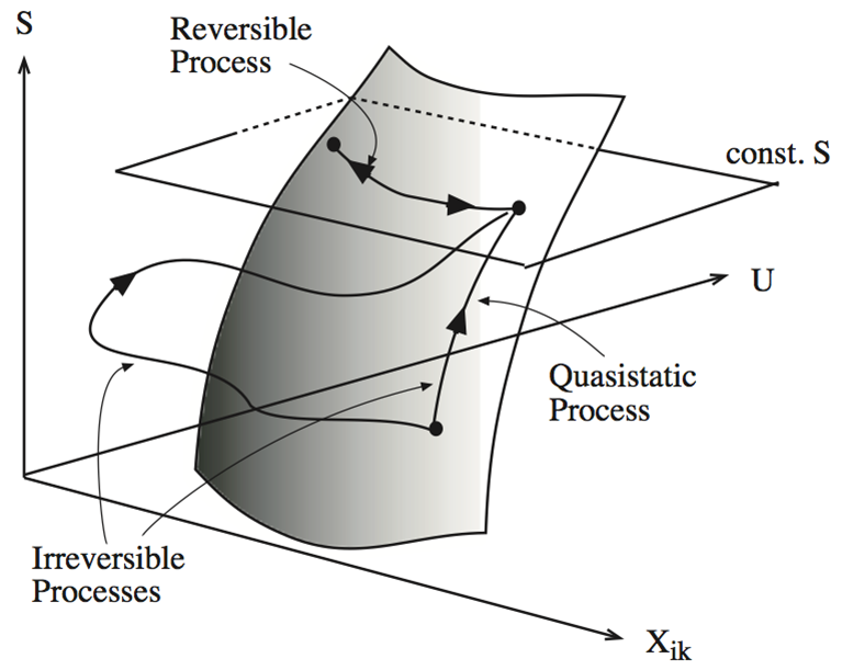
Fig. 5.1: Irreversible, quasistatic and reversible processes
Thermodynamics only makes statements about equilibrium states, when the fundamental equation is satisfied. However, by using quasistatic and reversible processes as idealized limits, we can derive inequalities satisfied by real processes.
As seen earlier \(dU = đQ + TdS\) for small (quasistatic) heat transfers in absence of work. The best we can do in the presence of work is therefore that all of
\[ dU = Tds - pdV + \sum_i \mu_idn_i + \Gamma \,dA + H\,dM + ...\]
goes into work except for the first term, which corresponds to the infinitesimal heat transfer. \(–PdV\) would be simple bulk volume work (e.g. expansion of a gas), \( H dM\) would be chemical work (e.g. electrochemical if \(n\) refers to the mole number of an ion), \(\Gamma dA\) would be surface tension work (e.g. blowing a soap bubble), \(H dM\) would be magnetic work, etc.
The heat transfer cannot be reduced below \(TdS\). However, part or all of the energy flow \(đW\) can of course be converted to heat \(đQ_W\). The entropy will rise further by \(T\,dS_W=đQ_W\), and correspondingly less work is done:
\[ dU=TdS + đQ_W + đW_{\text{left over}}\]
If all possible work is converted to heat, \(đW_{\text{left over}}=0\) and heat flow is maximized. The following theorem tells us how much work at most we can extract from a system.